Tutorial Zonal Statistics and Area Computations

4.1. Style a continuous raster

Make sure you see the project with layers subcatchment and DEM visible in the map canvas. In this chapter we'll only work with those layers.

Let's first style the Digital Elevation Model (DEM) so we can clearer see the value range.

The default legends produced by Desktop GIS software are often not intuitive, because the software does not know (1) what information is presented, and (2) the raster data type (e.g. Boolean, discrete or continuous data). To help interpret the results it is good practice to style your layers intuitively.

The DEM is a continuous raster. Continuous rasters represent gradients and can therefore contain real numbers (or floating point). Continuous rasters are styled in QGIS using ramps in the Singleband pseudocolor dialogue.

1. Select the DEM layer and click  to open the Layer Styling panel (or press F7).

2. In the Layer Styling panel choose Singleband pseudocolor from the drop-down list.

3. Right-click on the color ramp and choose Create New Color Ramp.

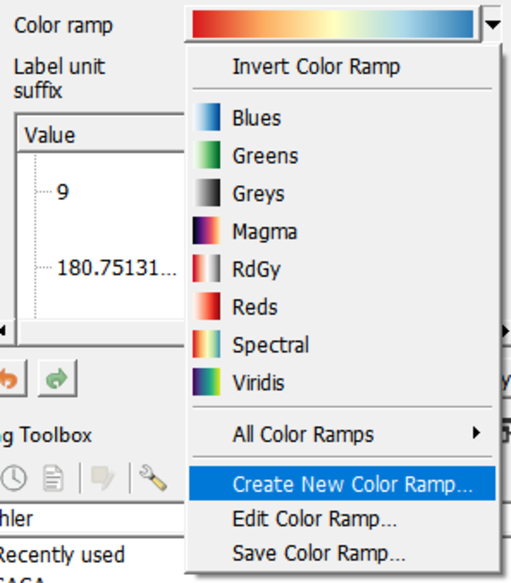
4. In the popup Color ramp type dialogue choose Catalog: cpt-city from the drop-down list and click OK.

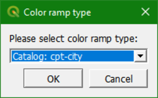
The cpt-city catalogue has a lot of useful preset color ramps.

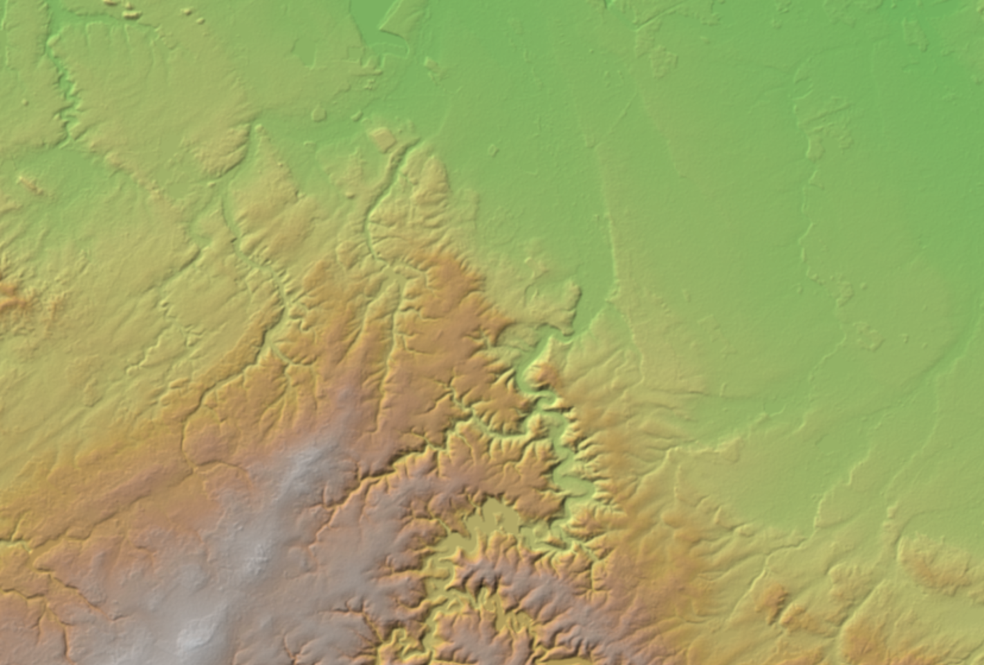
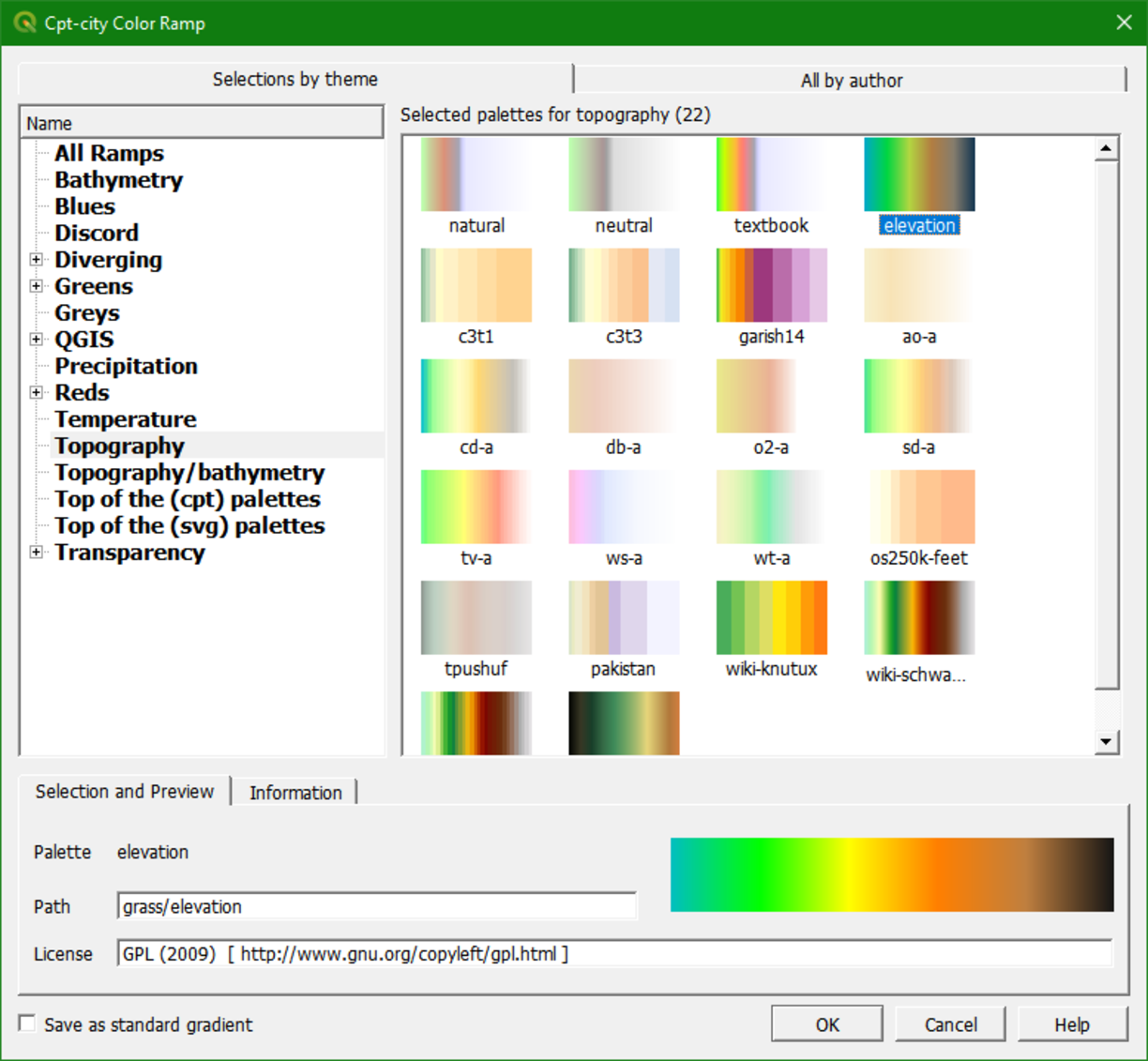
5. Choose Topography | Elevation. Note that cd-a and sd-a are also nice choices. Click Classify in the Layer Styling panel to apply the ramp.

This gives us more intuitive colors in the DEM where we can clearly distinguish higher and lower areas. Now we will further improve the visualisation.

6. Right-click on the DEM layer in the Layers panel and select Duplicate Layer.

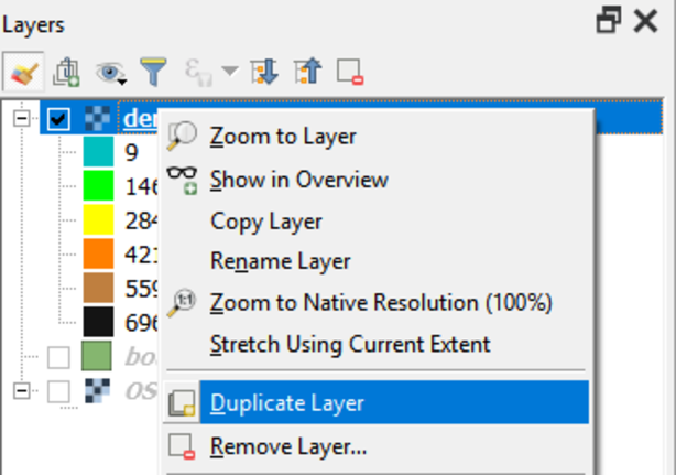
This creates a copy of the DEM layer called DEM copy.

7. Uncheck the DEM layer, check DEM copy and rename the layer to hillshade.

8. In the Layer Styling panel, which should still be open, make sure that the hillshade layer is now selected. In the drop-down list change Singleband pseudocolor to Hillshade.

Now the hillshade layer is visualised with a shading.

Which direction is the illumination coming from? Is this possible in reality?

Hillshade gives the best results with an artificial illumination in the northwest, which in reality can not exist in the Northern Hemisphere. If you move the dial in the Layer Styling panel to the southwest, you will see an inverted relief. Also note that there is a Resampling section. The default resampling method for both Zoomed in and Zoomed out is Nearest Neighbor. This method is fine for categorical data however, elevation is considered continuous data. You should therefore choose a Zoomed in resampling method of Bilinear and a Zoomed out resampling method of Cubic.

Next, we're going to blend the DEM with the hillshade layer.

9. Switch on the DEM layer by checking the box.

10. In the Layer Styling panel make sure the dem_fill layer is selected. In the Layer Rendering block of the panel, change the Blending mode to Multiply.

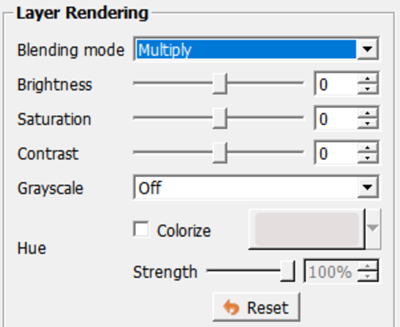
As you can see, blending gives a much nicer effect than transparency. With transparency the colours will fade. Now we can clearly see the elevation differences: the gradient from south to north and the valleys where we expect the streams.