Fire Risk Map

2.4. Land Cover

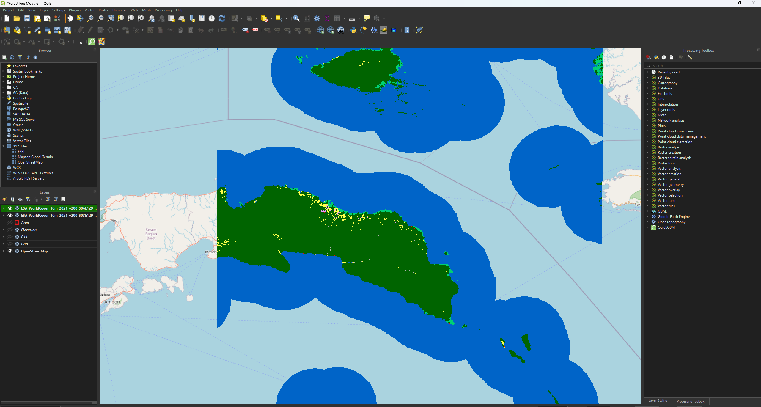
The WorldCover map from the ESA shows all the land cover types that you can encounter in the world. Think of forests, agriculture, cities, oceans, etc. This gives you a quick overview of what the landscape looks like, which can sometimes be a bit difficult if you’re using satellite imagery. The WorldCover map is in a 10m resolution and created from Sentinel-1 and Sentinel-2 data. While very useful, it’s good to remember that the map may not always be fully accurate. Of course, you can create your own land cover map using satellite imagery and machine learning, but this is quite a tricky job, which we won’t do during this module.

 If you haven't dowloaded the data yet, you can download the Land Cover data here.

Reprojecting

Much like the previous layers, we need to Reproject these layers as well. Make sure you have both the ESA_WorldCover_10m_2021_v200_S03E129_Map.tif and ESA_WorldCover_10m_2021_v200_S06E129_Map.tif layers.

1. Open the Warp (reproject) tool.

3. Set the Target CRS on EPSG: 32752.

4. Set Resampling method to use on Mode.

For this Resample, we use Mode, as it works the best for categorical data, like our World Cover map. We don’t want to get an average of the values here as we did with the satellite imagery.

5. You can save the Permanent layers as WorldCover_Reprojected_1.

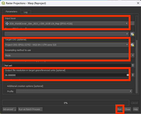
6. Once finished, check if the projection is correctly set on EPSG: 32752 and 30 by 30 pixels.

7. Repeat the same steps for the other WorldCover layer. Save it as WorldCover_Reprojected_2.

 

Merging Data

As you will often see, the data is split up exactly at the location we want to use, forcing us to download two layers of data. Luckily, we can combine the data to make one layer instead, which will make our work a lot easier later on.

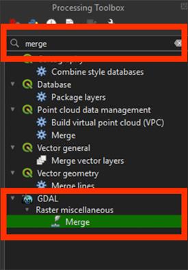
1. Go to the Processing Toolbox. Search for Merge under GDAL > Raster miscellaneous. Double click to open the tool.

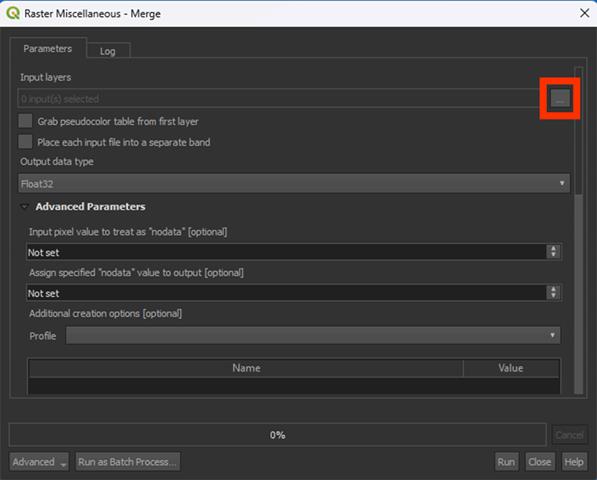
2. By Input layers, press the ‘…’ button.

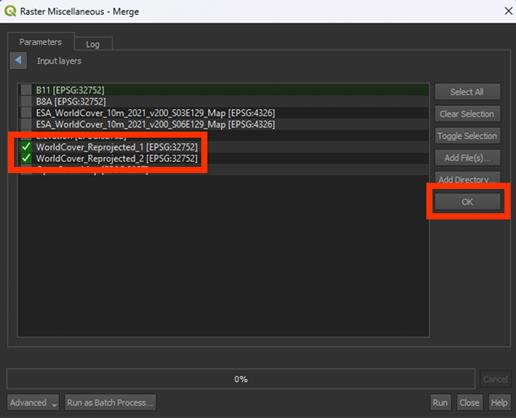
3. Select the WorldCover_Reprojected_1 and layers WorldCover_Reprojected_2 layers that we want to combine, then press OK

4. Run the tool. We don’t need to save a Permanent layer.

Note: This may take a while if they layers are large. You may want to clip the layers first if your hardware is having trouble.

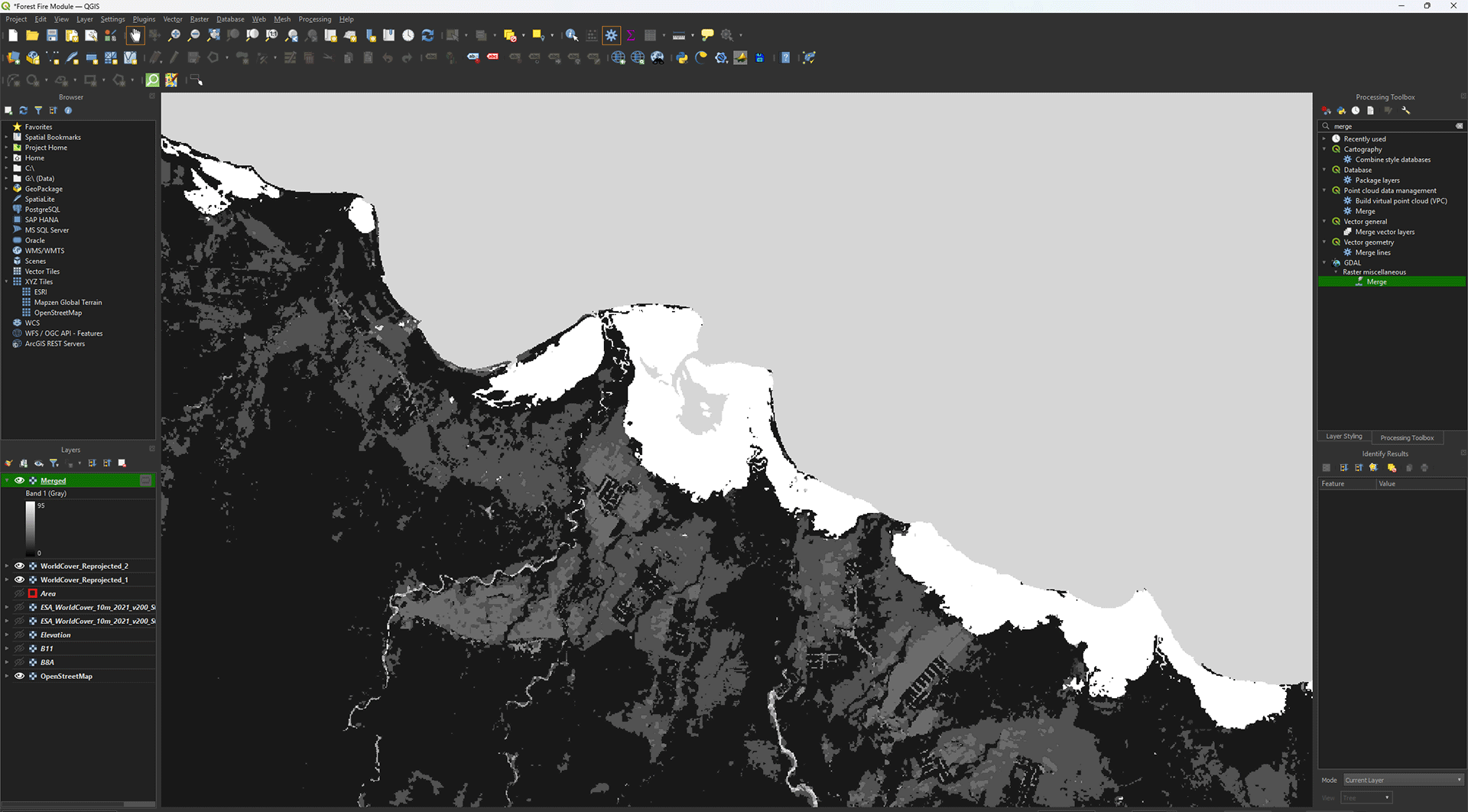
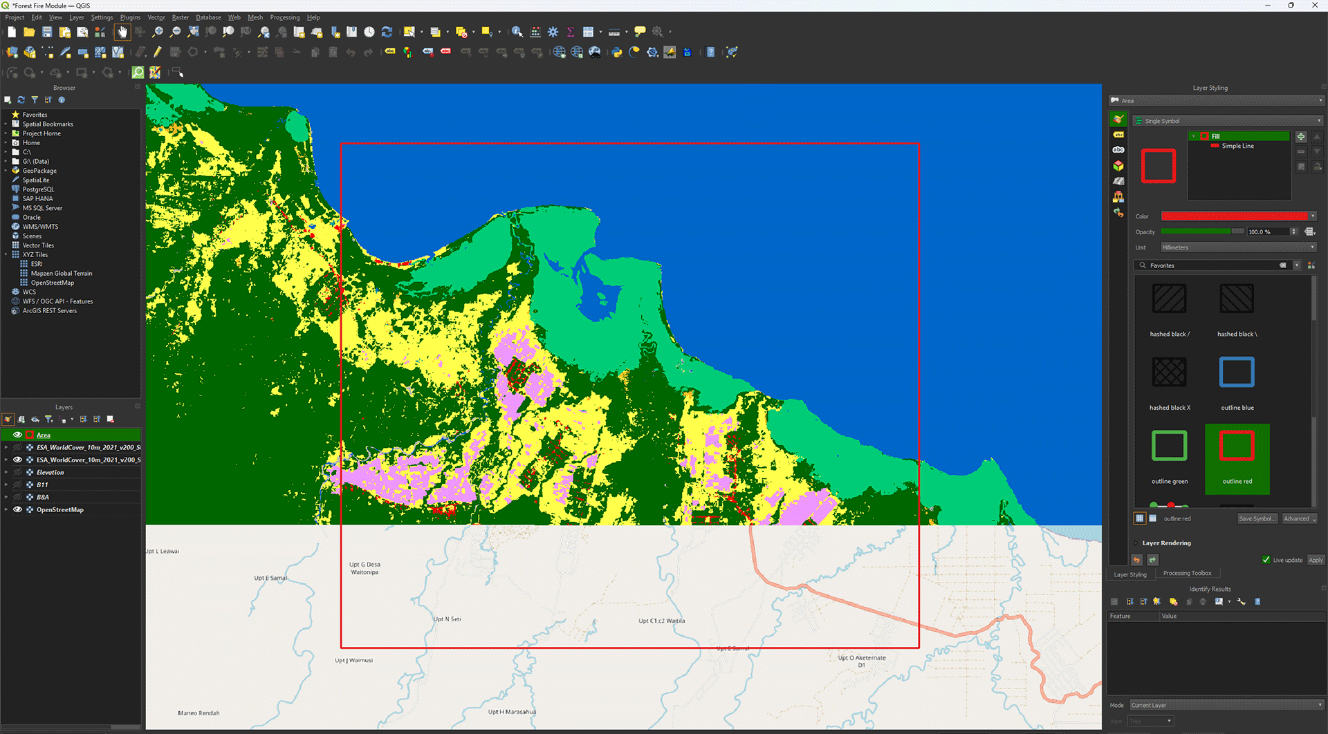
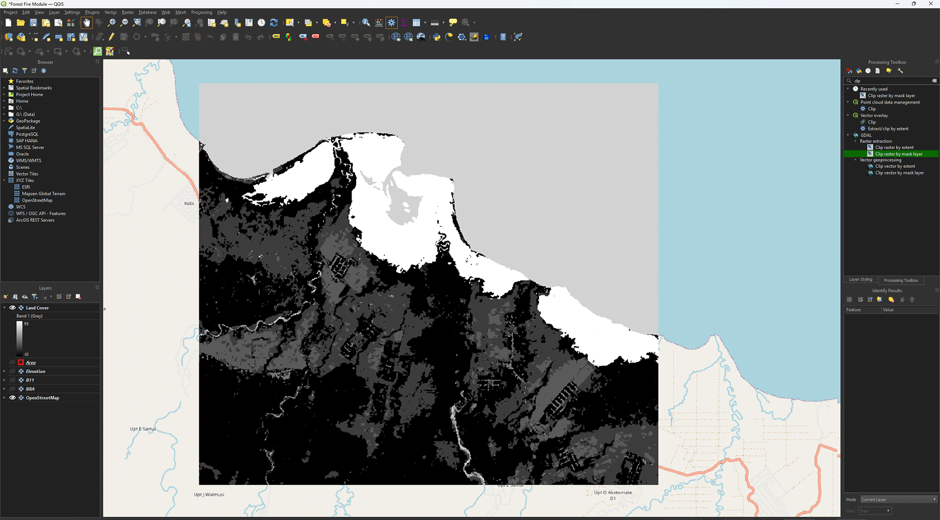
Suddenly the layer is in greyscale. Before we change the symbology, however, we will clip the area into our study area if you haven’t done that yet.

4. Clip the area using the same process as before, with the Clip raster by mask layer tool. Save the Permanent layer as LandCover, then delete the Merged layer, reprojected layers, and original WorldCover layers we imported.

 

Symbology

You might have noticed earlier that the symbology of the layers was complete nonsense when we first imported the data. We need to add a QML-file to get the correct symbology to show up. You can find the QML-file if you click on the Information icon on the WorldCover website or by using this link: https://esa-worldcover.org/en/data-access. If you downloaded the data from the module, the QML-file should be in your folder.

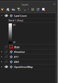
1. Right click on the Land Cover layer > Properties > Symbology.

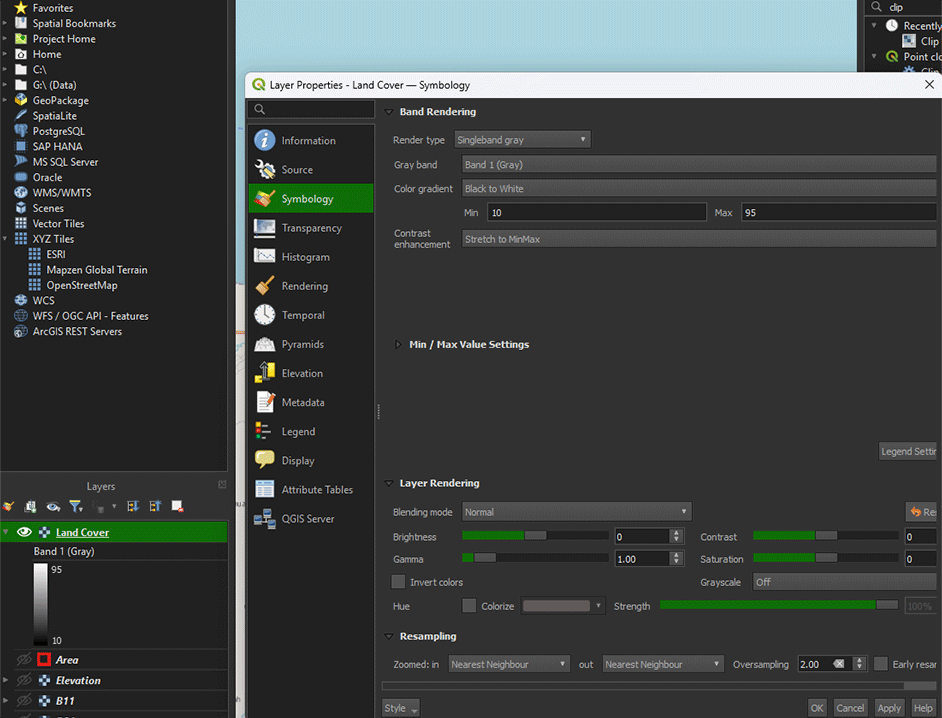
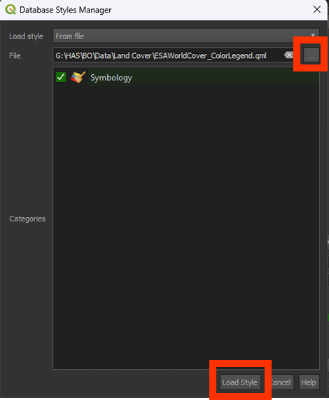
2. Go to the Style button and select Load Style.

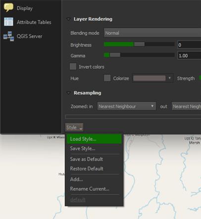
3. In the new window, click on the ‘…’ button and load the QML-file you just downloaded. Once loaded, click on Load Style.

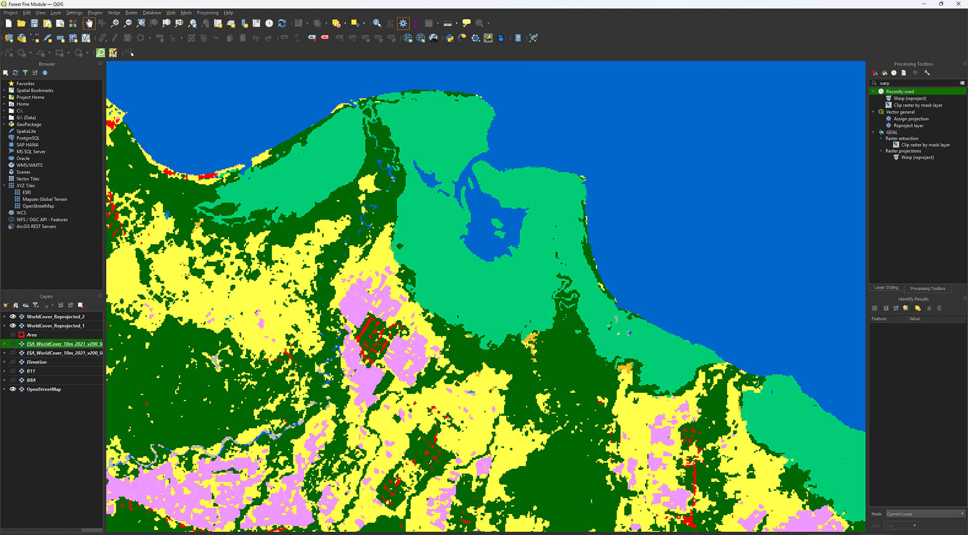
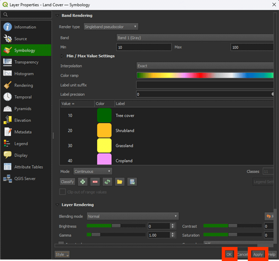
The Merged layer should now update with the correct symbology

4. Click Apply and then OK on the Properties window.

Now that we have the imported the WorldCover data, we can see what the land cover types are in the study area. It’s quite varied, which will lead us to interesting results once we start analyzing.

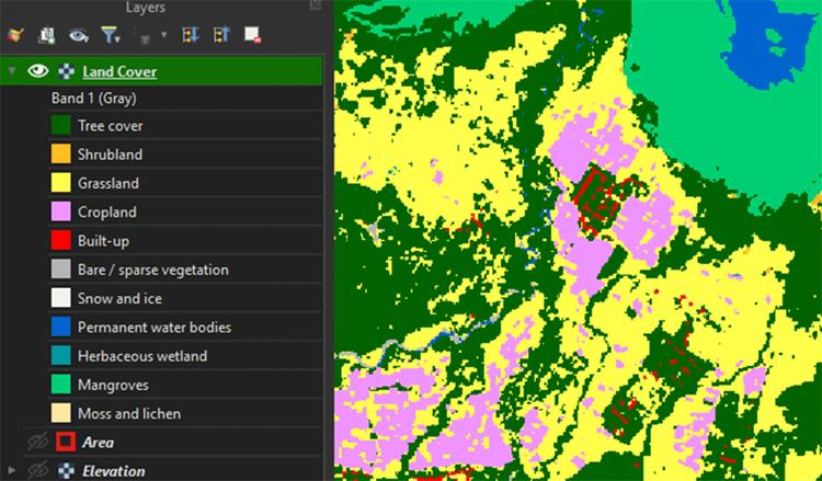
You have reprojected, merged, and visualized the Land Cover layer. Don’t forget to save your project before continuing.