Fire Risk Map

3.3. Distance to Built-Up Area

We downloaded vector layers of the roads and buildings in our study area. Fires often start near human activity, so we want to take that into account for our analysis. The closer an area is to human settlements, the more susceptible it is to fire. Creating a buffer around the roads and buildings will show which areas on the map are in close proximity to them, and thus at risk.

Buffer

Note: The buffer calculation can be very heavy and time-consuming for lower powered devices. This is one way to create a ringed buffer, but you can also use a different method we will cover when creating the Buildings buffer. If you cannot complete the roads buffer, you can use the buildings buffer steps and create the roads buffer that way. Make sure that you use the correct values and layer names!

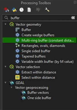
1. Go to the Processing Toolbox and search for Multi-ring buffer (constant distance) under Vector geometry. Double click to open the tool.

For our buffer, we want to create four classes of the same distance. We will start with the Roads layer, which will have a buffer of 1200 meters. The Multi-ring buffer makes this very easy to do.

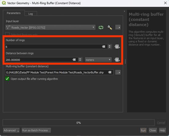
2. In the Multi-Ring Buffer window, select the Roads layers as the Input.

3. Under Number of rings, choose 6. This will give the number of rings (classes) we want.

4. Under Distance between rings, set it on 200 meters. The tool will create 6 rings that are all 200 meters wide. As we chose 6 rings, we get a buffer of 1200 meters.

5. Save the Permanent layer as Roads_VectorBuffer.

6. Run the tool

Now we have a buffered layer that has 6 rings of 200 meters.

 

 

Symbology

While not a necessary step, we can change the symbology to check if our buffer was created correctly.

1. Go to the Layer Styling Panel and set the Render Type to Categorized.

2. Set Value on distance.

3. Click the Classify button to create the classes.

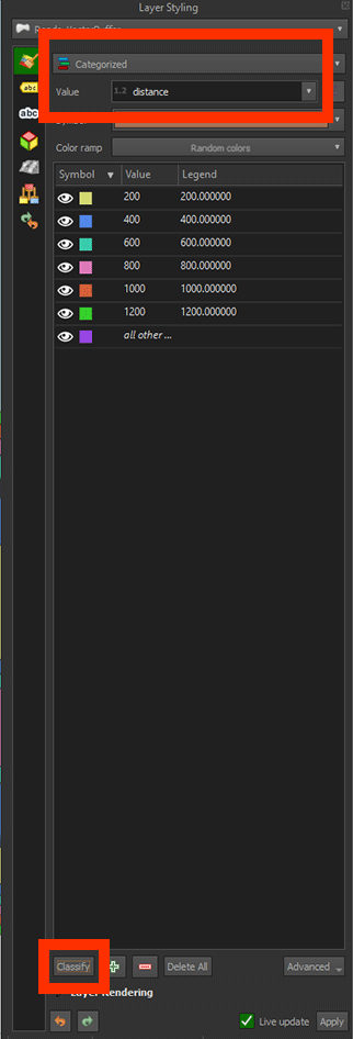
Now we can see that the buffer shows colours based on the value we gave before. Every colour is a width of 200 meters, neatly categorised.

If you click on the Identify Features button (ctrl + shift+ i), you can click on the buffers to see their values. A panel will open named Identify Results. Look at distance and it should show the buffer’s value, in this case ring 6, which is 1200 meters.

Converting the Vectors to a Raster

The buffer is created, but we can’t use it for our analysis just yet. All our other layers are rasters, but this one is still made of vectors. We will need to convert them.

 

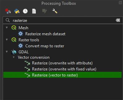
1. Go to the Processing Toolbox and search for Rasterize (vector to raster) under GDAL > Vector conversion.

In the Vector Conversion window, you'll need to enter values for width and height. So, before we continue, it's important to use the same values from the other layers. This ensures that the pixel size and extent of the raster match exactly. Luckily, we used an Area polygon to cut them to the same size.

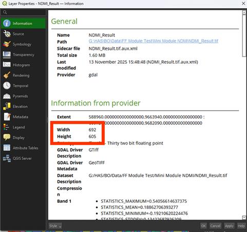
2. Right click the NDMI_Results layer > Properties (you don’t need to close the Rasterize window).

3. Go to the Information tab.

In the Information tab you'll see the width and height of the layer, which is what we’re interested in. In this case, the width is 692 pixels, and the height is 605 pixels. Keep in mind these values may be different for you, so make sure to write down your own values somewhere to use later.

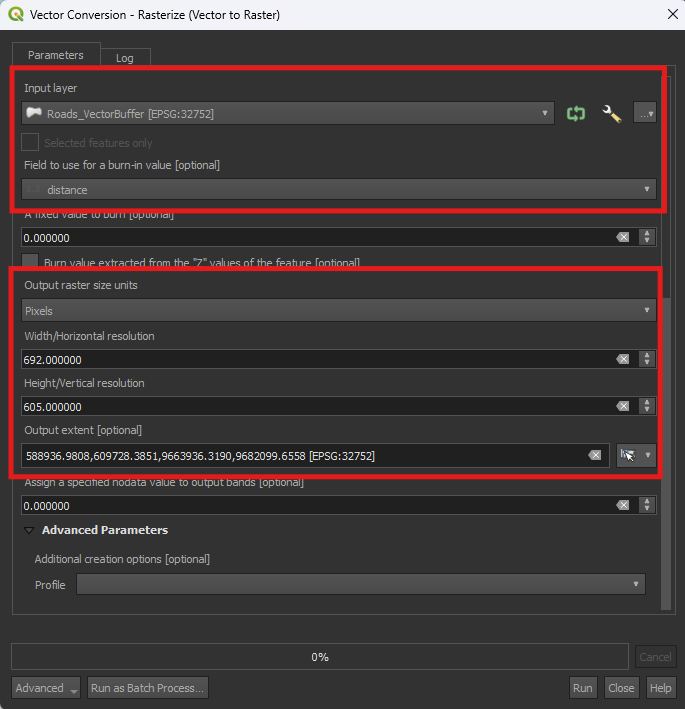
4. Close the Properties window. In the Rasterize window, make sure that Roads_VectorBuffer is set under the Input layer.

5. Set Field to use for a burn-in value to Distance. This will use the six ringed values we created earlier.

6.  Set Output raster size units to Pixels.

7. Set the both Width/Horizontal resolution to your width and length you looked up earlier. The width goes in the top box and the height in the bottom one.

In the case of this example the Width is set to 692 and the Height to 605. Your values may differ. Use the values you’ve written down earlier and type them in.

8. Click the arrow next to the Output extent > Calculate from Layer > Area.

9. For now, we don’t need to save it as a Permanent layer, so you can Run the tool.

If you zoom in, you'll see that the river layer has been converted into a raster. Instead of lines, it now consists of individual pixels, just like the other layers we created. However, there is still some empty data, which we will need to fill.

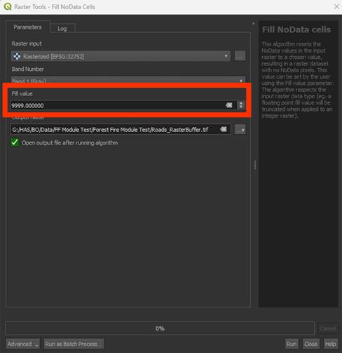
10. Open the Processing Toolbox and search for the Fill Nodata cells tool we used earlier. Make sure the Rasterized layer is used as the Input.

11. Set Fill value on 9999.

12. Save the Permanent layer as Roads_RasterBuffer and Run the tool.

The result looks a bit weird, as the individual rings seem to be gone.

13. Go to the Layer styling panel, set the Render Type to Paletted/Unique values and press the Classify button.

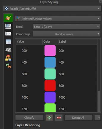
You should now see the individual rings again, with the empty areas filled in with a 9999 value (yellow in the example).

You can delete the Temporary Rasterized layer.

 

Buildings

For the buildings, we're going to use a different method to get a similar result. The method we used for the Roads works well, but with large datasets, like our buildings layer, it can be quite heavy to run. As we want to do this in a reasonable time, we'll use a lighter way to create the Multi-ring buffers using the Proximity tool. First, however, we need to convert the vector to a raster.

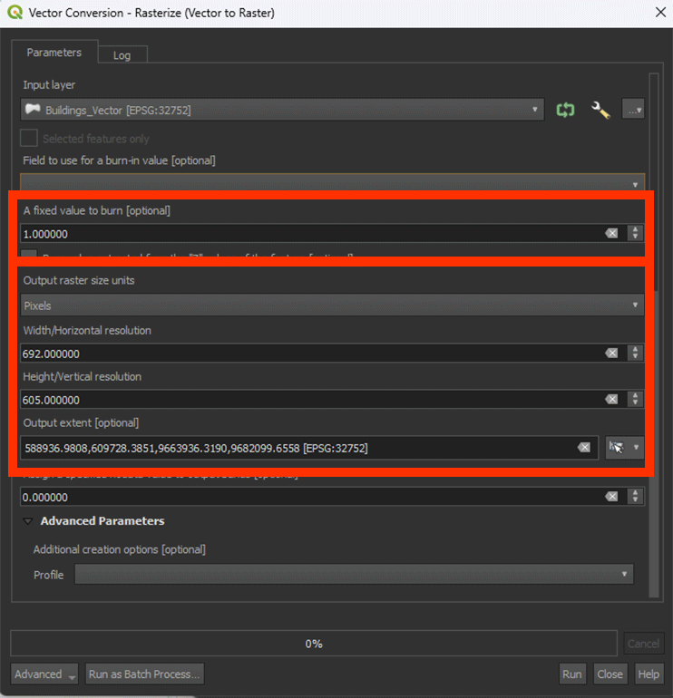
1. Open the Rasterize (vector to raster) tool again.

2. In the Rasterize window, make sure Set A fixed value to burn is set to 1. We need to use this now as we don’t have a field to use like we did with the Roads buffer.

3. Set Output raster size units to Pixels.

4. Set the Width/Horizontal resolution and Height/Vertical Resolution, using the same values as before.

5. Click the arrow next to the Output extent > Calculate from Layer > Area.

6. You don’t have to save it as a Permanent layer, so you can Run the tool.

We have converted the vector layer to a raster. This will make the buffer analysis a lot less heavy on processing.

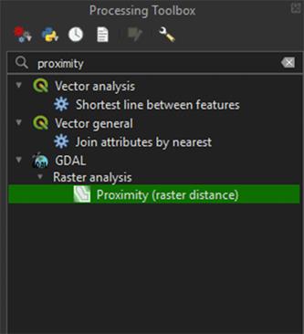
7. Go to the Processing Toolbox and search for Proximity (raster distance) under GDAL > Raster analysis. Double click to open the tool.

Much like the Multiring buffer tool, Proximity lets us create a buffer around the Buildings. However, we can’t create the six rings as before, so we need to Reclassify later.

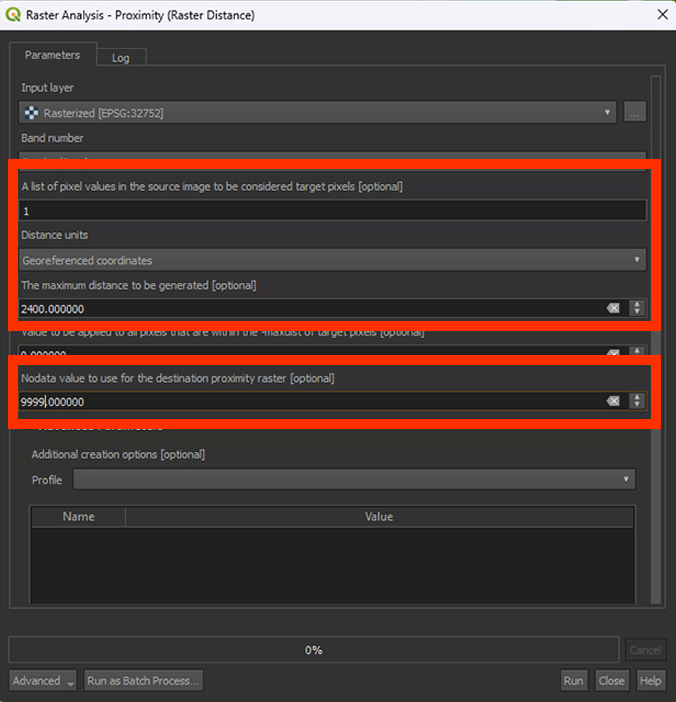
8. Make sure you have the Rasterized layer selected.

9. Set A list of pixel values in the source image to be considered target pixels to 1. This will make sure that the buffer is created around the buildings.

10. Set Distance units on Georeferenced coordinates.

11. Set The maximum distance to be generated to 2400. This is necessary to create our buffer of 2400 meters.

12. Set Nodata value to use for the destination proximity raster to 9999. Everything past the 2400 meters will get a 9999 value.

13. Save the Permanent layer as Buildings_RasterBuffer and Run the tool

You can delete the Temporary Rasterized layer.

We get a result that looks a bit different from the clean buffers we created for the Roads layer. However, if you click around with the Identify Features, you can see that the values are nicely between 0 and 2400. Everything further than 2400 meters gets a value of 9999. For now, we are finished with this layer. In 4.4 Roads and Buildings, we will Reclassify the layers, which will neatly categorise everything back into ringed buffers.

We finished the analyses. Save your project and we will continue with the Weighted Overlay Analysis in chapter 4.