Fire Risk Map

4.5. Calculate Fire Risk Map

All layers are now reclassified, which means we can perform the Weighted Overlay Analysis.
For this, we use the Raster Calculator, where we can enter different formulas to perform calculations with map layers.

During this analysis, we overlay all the layers, and the final score will be calculated for each pixel, resulting in values between 0 and 10. We also assign a weight to each layer, depending on which layer is more important for our analysis. For example, NDMI is given more weight than the Slope, because the moisture in the vegetation is a more important factor for fire risk than the landscape’s slopes.

 

Raster Calculator

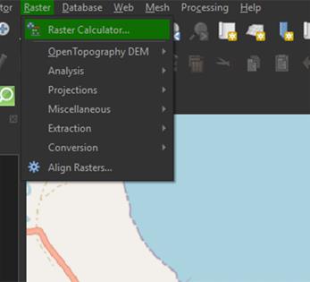
1. In the top menu, go to Raster > Raster Calculator.

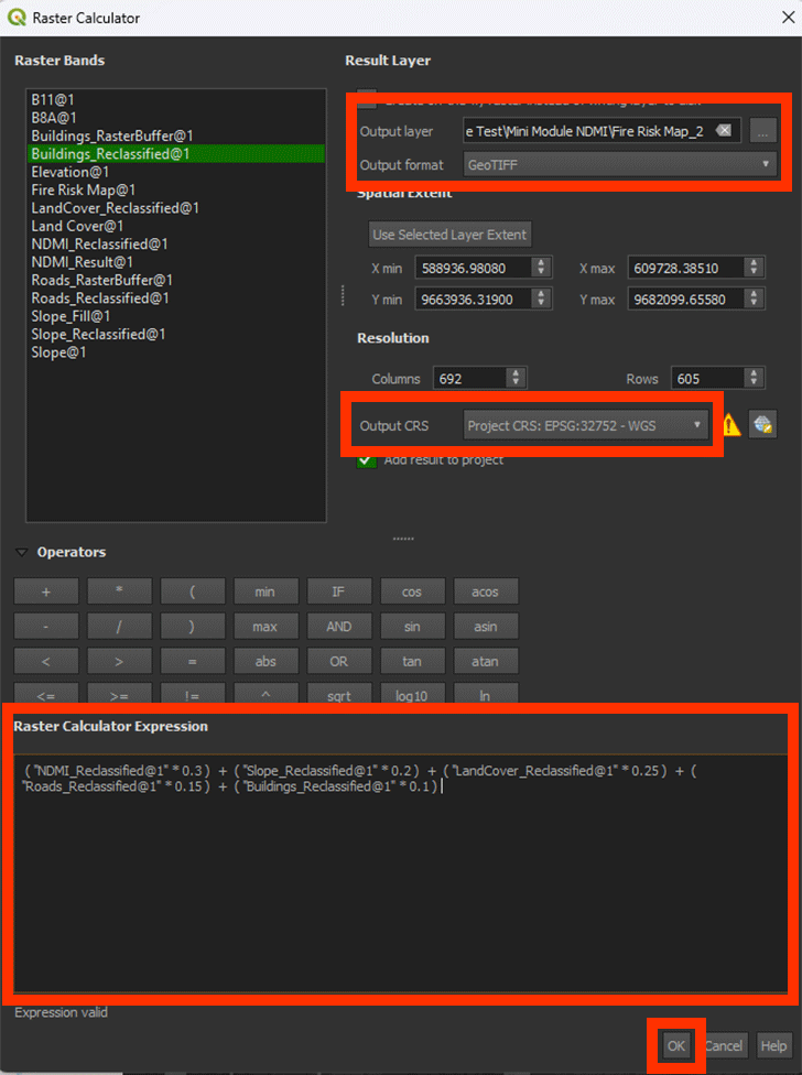
2. In the Raster Calculator Expression field, enter the following formula:

( "NDMI_Reclassified@1" * 0.3 ) + ( "Slope_Reclassified@1" * 0.2 ) + ( "LandCover_Reclassified@1" * 0.25 ) + ( "Roads_Reclassified@1" * 0.15 ) + ( "Buildings_Reclassified@1" * 0.1 )

Note: If you have renamed the layers, you should use those names in the formula. You can double-click on a layer in the Raster bands section to insert it directly into the formula. If the formula is correct, you should see Expression valid left under the Raster Calculation Expression box. If it says Expression Invalid, you can check if all the brackets are added in the right place, or if you used commas instead of periods, it should be periods.

3. For Output layer, save the layer as Fire Risk Map by clicking on the ‘…’ button.

4. Ensure the Output CRS is set to EPSG:32752.

5. Click OK to calculate the risk map layer.

With this formula, we calculate the sum of all the pixel’s values that overlap, in this case it being five map layers. With the values we add in the formula, we can add how important the layer is to the formula with weighting. In other words, what is a larger factor contributing to fire risk? In the table below you can see the ranking of the weights we use. These can always differ depending on your research and what you want to calculate.

Layer	Weights
NDMI	0.3
Slope	0.2
Land Cover	0.25
Roads	0.15
Buildings	0.1

 

The weights given to each layer have been calculated using the AHP-method. This is a reliable way of giving weight to certain unquantifiable variables. It is also a widely used method for forest fire mapping. For more information about how to calculate it yourself, you can look into this paper:

The weight should always add up to be a value of 1, or 100%. The Land Cover map, for example, counts for 25% in our calculation.

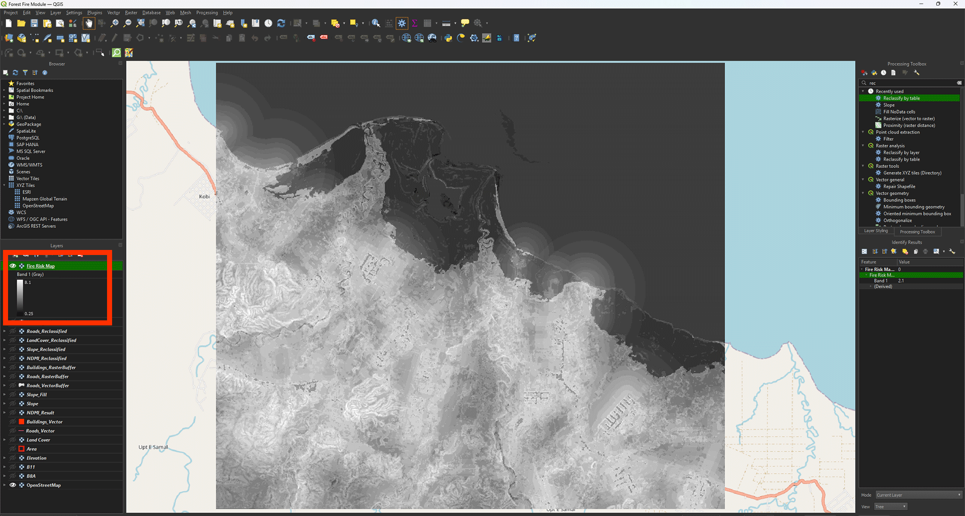
Now, we finally have our Fire Risk Map. You can see the colours represent how high the score ended up being. If everything went correctly, the value should be between 0 and 10, in this case its 0.25 and 8.1 for the example. The higher the score, the bigger the fire risk. Most of it is located around the crop- and grassland. This is a reasonable result, when looking at the research done beforehand.

 

Symbology

 We can give it some colour to make it a bit more clear.

1. Go to the Layer Styling panel and set the Render type to Singleband pseudocolor.

2. Set the Color ramp on Reds.

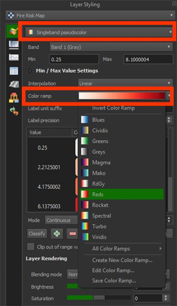
Now we can see the darker red areas having a higher risk for fires.

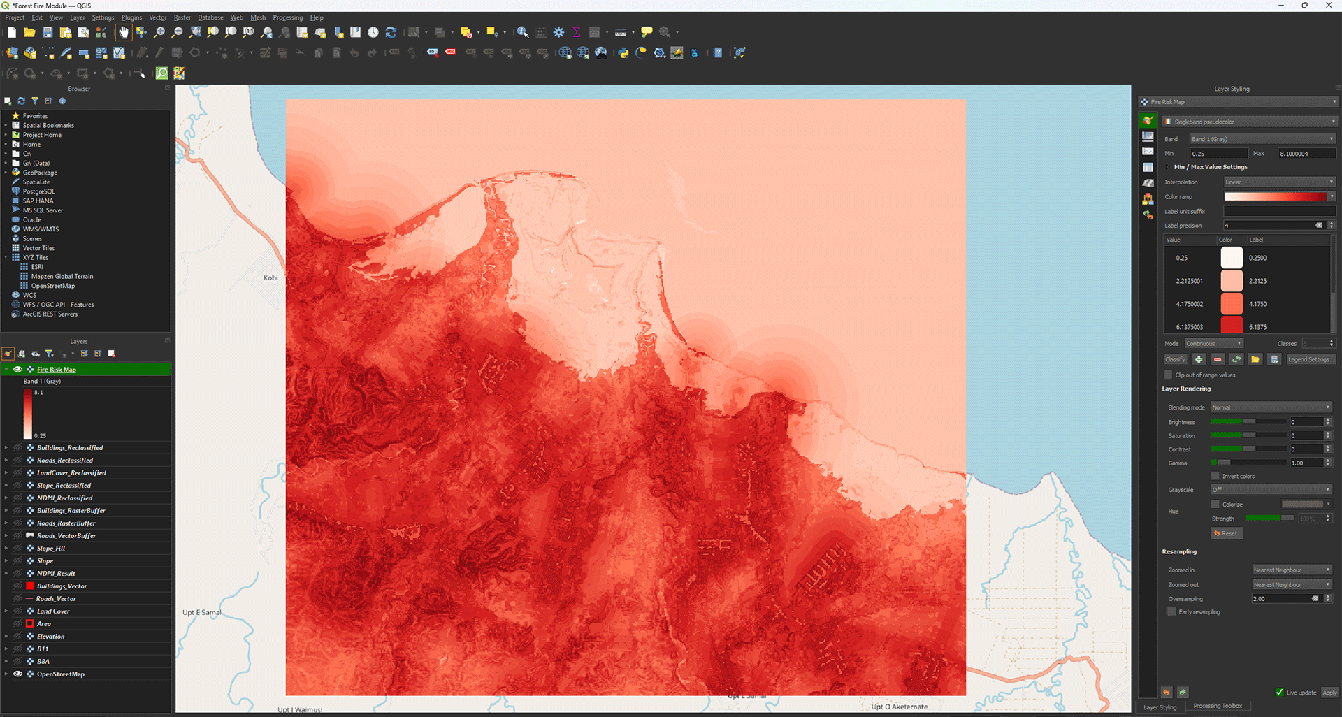
Even though it gives us an idea of what areas are susceptible to fires, the map itself is a bit messy. We can make a better, more usable overview.

 

Reclassify Risk Map

We want to get an easier overview of which areas are at most risk of fires starting. Knowing this, we could use the map to start mitigating and preventing fires in the future. To do this, we will convert the raster we created to a vector layer using grids.

1. First, we will use the Reclassify tool again. Go to the Processing Toolbox and open the Reclassify tool.

2. Make sure the Fire Risk Map is set as the input.

There are many different ways we can categorize our Fire Risk Map and it really depends on what you think is the best way. For this module, we will divide the score into 4 categories. 1 being low risk and 4 being high risk.

3. In the table, fill in the values down below and press OK:

Minimum	Maximum	Value
0	2.5	1
2.5	5	2
5	7.5	3
7.5	10	4

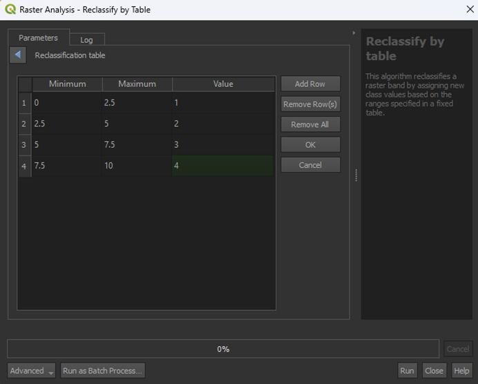
4. Save the Permanent layer as Fire Risk Map_Reclassified and Run the tool. Range boundaries can stay on min < value <= max.

TIP: Look closely at the options, you can easily select the wrong one by not picking the one with "<=" instead of just "<", this does matter.

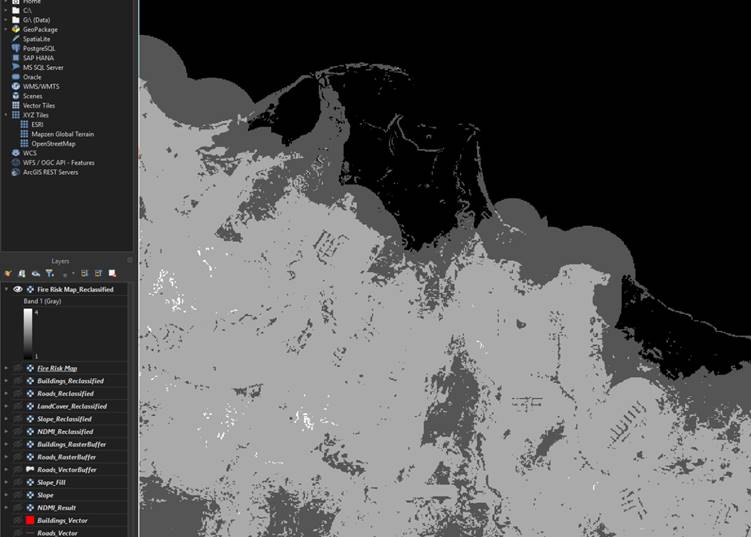
Now we have the Fire Risk Map with 4 categories, ranging from low to high risk. This is already a lot easier to read, but we can use a vector layer if we ever want to use it in the future, as you can overlay it on maps or insert more data than just the risk values. For this module, however, we will just make the vector layer.

 

Grid Map

We are going to make a grid and use the values from the Fire Risk Map_Reclassified to create a grid risk map.

1. Go to the Processing Toolbox and search for Create grid under Vector creation. Double click to open the tool.

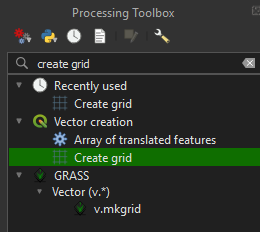
2. In the Create grid tool, set the Grid type to Rectangle (Polygon).

3. Click the arrow next to the Grid extend > Calculate from Layer > Area.

4. Set Horizontal and Vertical spacing on 1000 meters. We will get 1x1 kilometer sized grids, which fit well with our fairly small study area. The study area in the example is about 20x20 kilometers.

Note: Make really sure that the spacing is set on 1000 meters. If you run it when still set on 1 meter, it can crash your device.

5. Make sure the Grid CRS is set on EPSG: 32752.

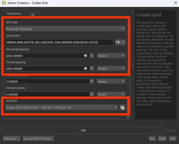
6. Run the tool. You don’t have to save a Permanent layer.

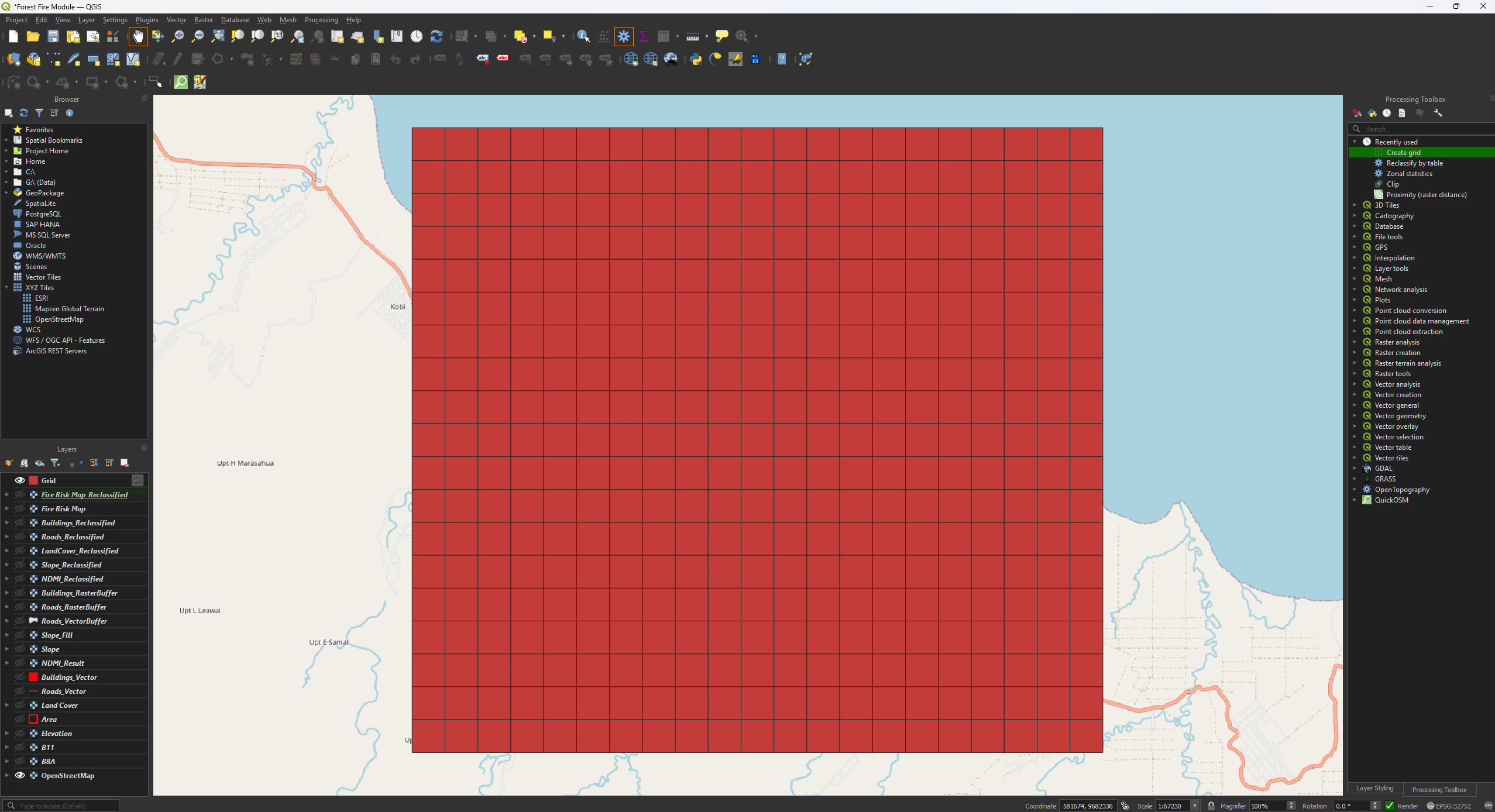
Now we have a nice grid, but it is larger than our study area. Let’s Clip the grid to the correct size.

7. Open the Clip tool, but this time the vector version. We are clipping a polygon, so use the Clip tool under Vector overlay. Make sure the Input layer is set on Grid.

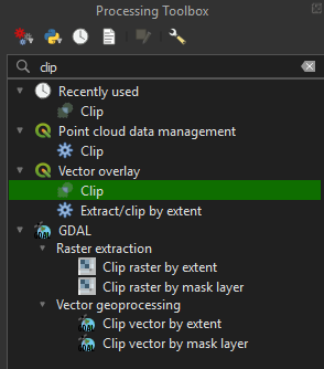
8. Set the Overlay layer on Area.

9. Run the tool. You don’t have to save a Permanent layer.

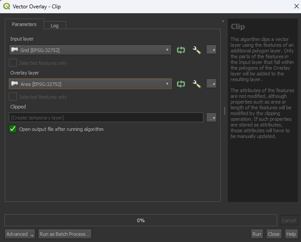
We now have a Clipped layer that is the same size as our study area.

Let’s put the risk categories into the grid we’ve just made.

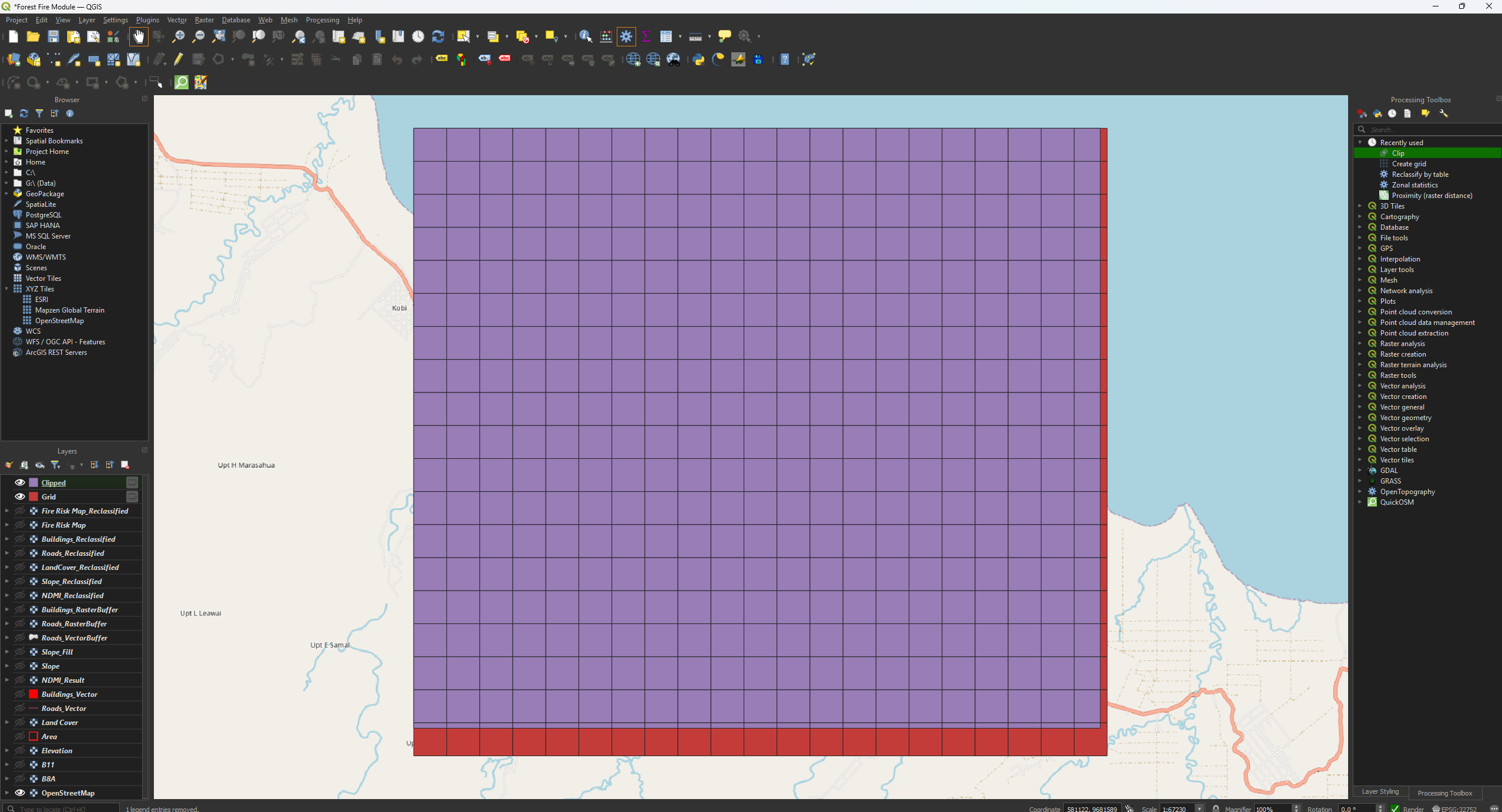
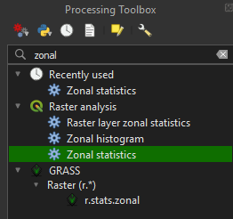
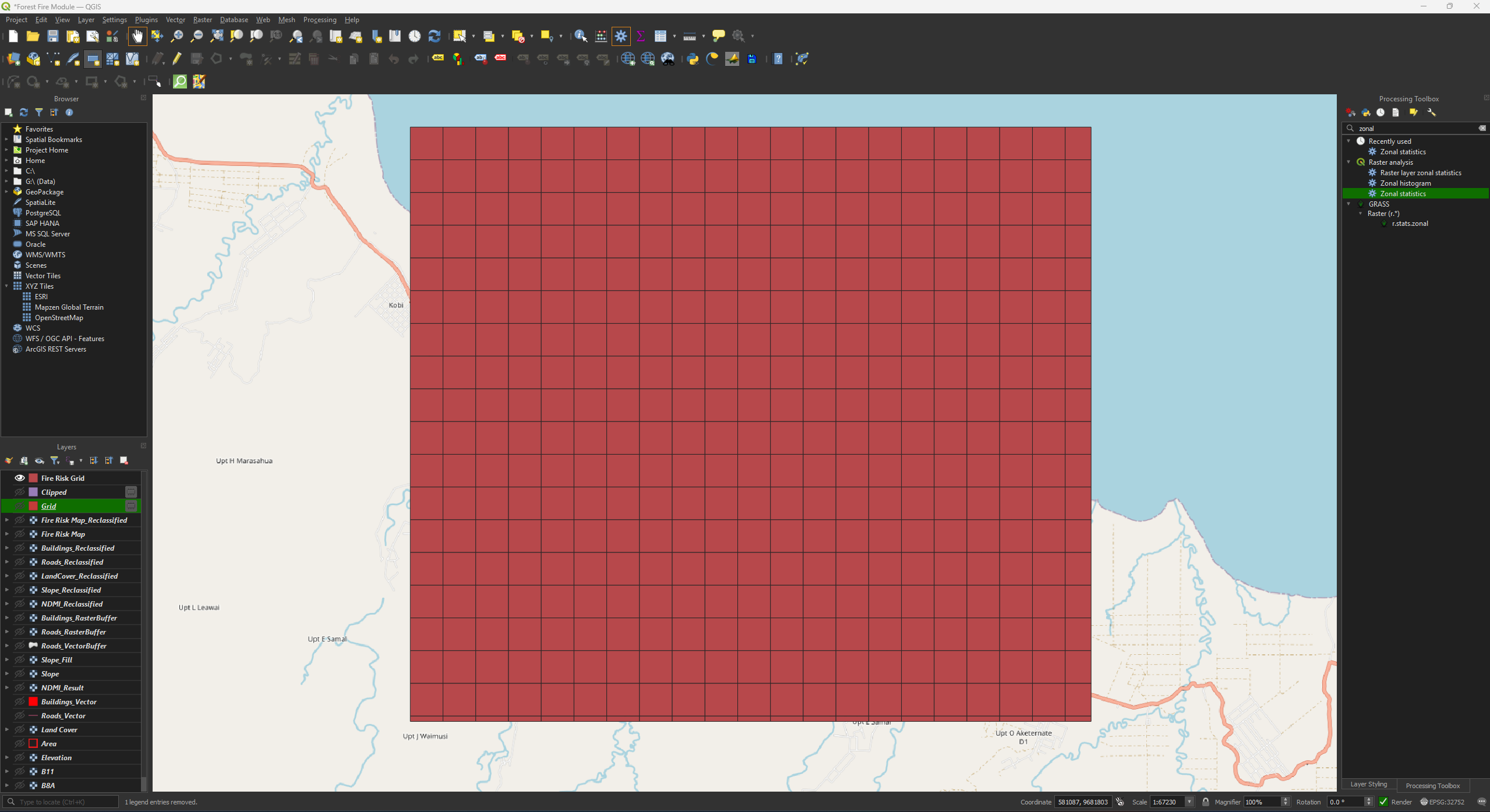
10. Go to the Processing Toolbox and search for Zonal statistics under Raster analysis. Double click to open the tool.

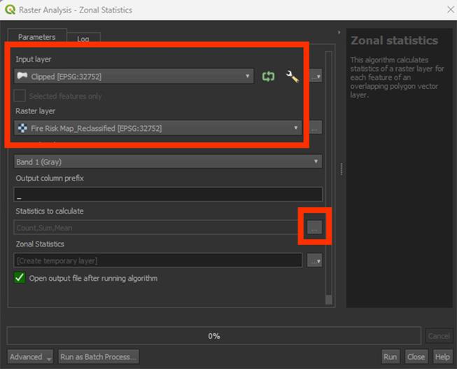
11. Make sure the Clipped layer is used as the input.

12. Make sure that the Fire Risk Map_Reclassified is used as the Raster layer.

13. Then, click on the ‘…’ button next to Statistic to calculate.

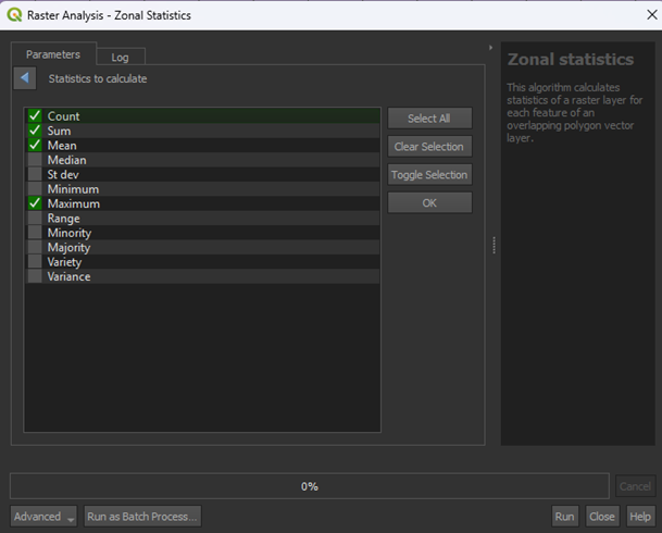
Here is the list of how the tool will calculate the values of the Fire Risk Map in the grid. Because we only have a value from 1 to 4, we will use Maximum. This will take the maximum value found from the Fire Risk Map in a grid cell and give the cell that value.

14. Select Maximum and press OK. You can leave the others on selected if they were already.

15. Save the Permanent layer as Fire Risk Grid (a SHP file) and Run the tool.

The Fire Risk Grid still has one colour. We need to adjust the symbology to get the final result. You can delete the temporary Grid and Clipped layers.

 

Final Symbology

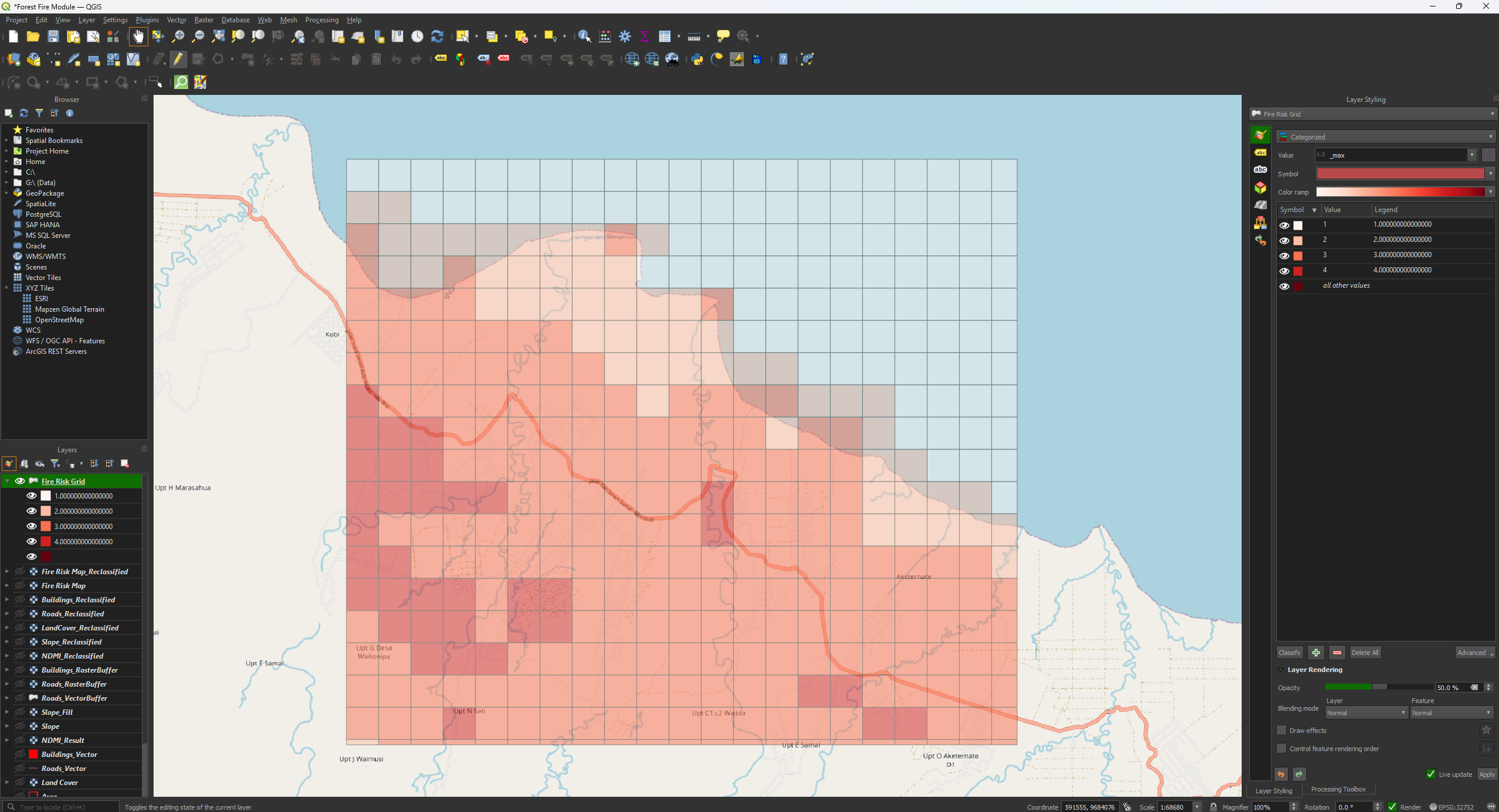
We have 4 values, 1 to 4. 1 is low risk and 4 is high risk. Let’s colour them accordingly.

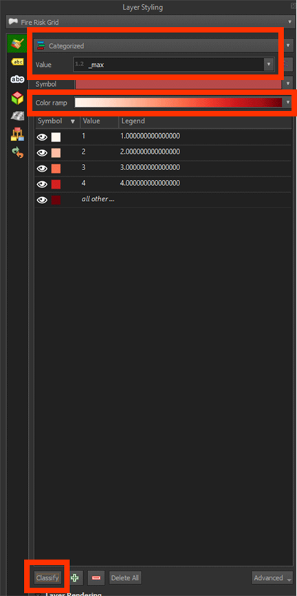
1. Go to the Layer Styling panel and set the Render type to Categorized.

2. Set the Value on _max. You may have to scroll down.

3. Set the Color ramp on Reds.

4. Press the Classify button.

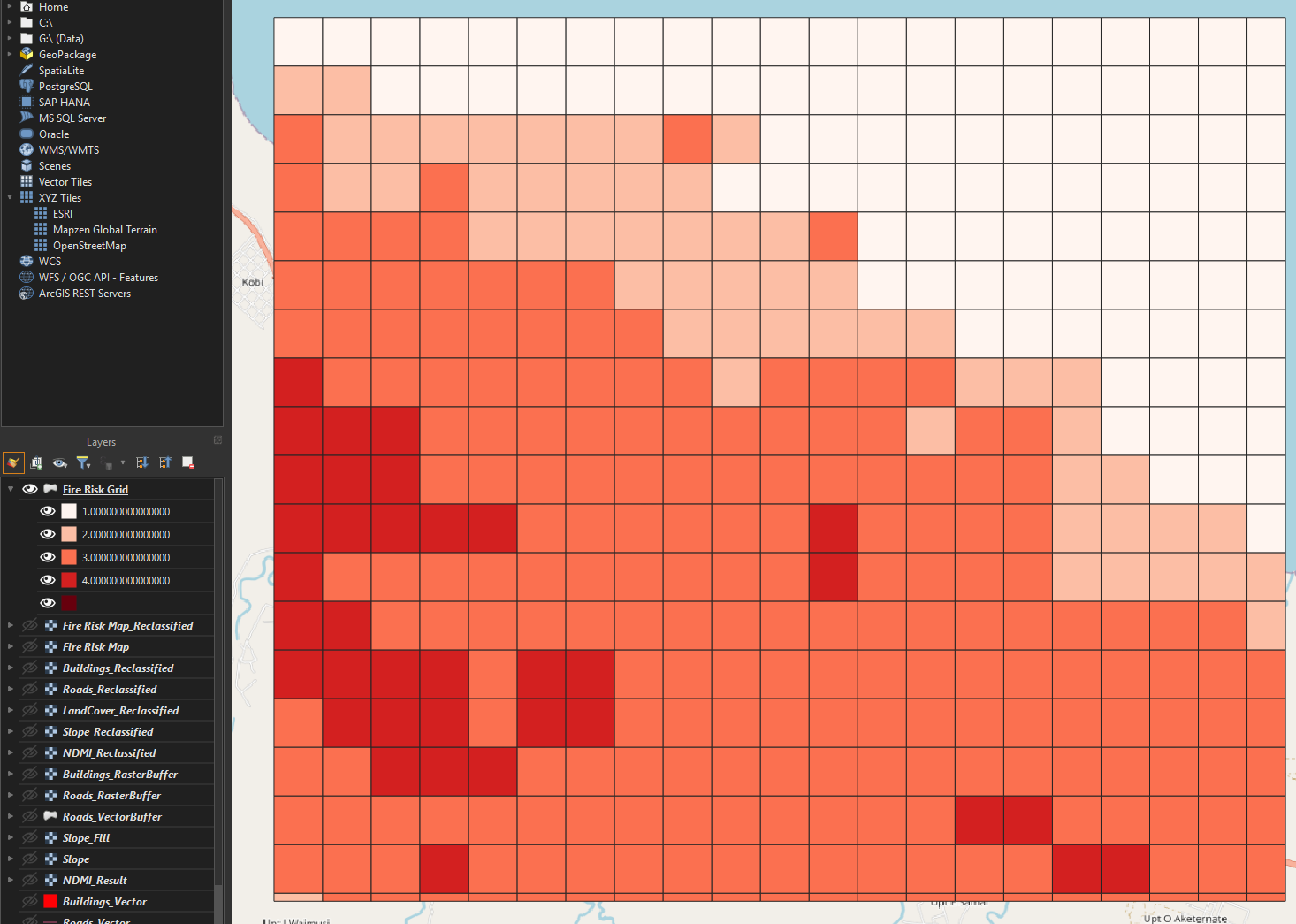
Now we have a grid with the categories. We can see that the biggest risk zones are found on the bottom left of our map. This map can show us what areas would have priority to look into for mitigating forest fires.

To make it a bit easier to see what the grid cells overlap, we can make the layer transparent.

5. Right click on the Fire Risk Grid layer and go to Properties. Then go to the Symbology tab.

6. Open the Layer Rendering tab and set the Opacity on 50%.

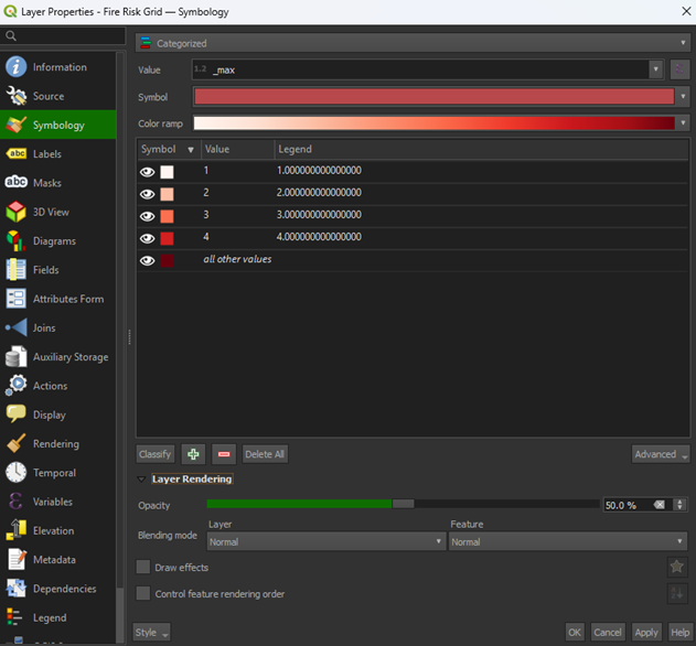
7. Press Apply and then OK to close the window.

If you have other layers open, hide them by pressing the Eye icons and only have the Fire Risk Map and OpenStreetMap layers open. Now we can see the basemap under our risk map. You could overlay this map over other data too and use it for future analyses.

You have now finished the Fire Risk Map. Make sure that you have saved the project before closing QGIS. If you want more practice with the tools and QGIS, take a look at the Extra Assignment which you can find after this chapter.