3D with QGIS and Aerialod
| Site: | OpenCourseWare for GIS |
| Cours: | Creating data visualisations with graphs, maps and animations |
| Livre: | 3D with QGIS and Aerialod |
| Imprimé par: | Visitante |
| Date: | samedi 20 juin 2026, 02:54 |
1. Introduction
Sometimes a visualization in 3D is clearer to tell your story than a 2D map. A 3D map or animation is often in 2.5D, where the 3D effect is created by shading and perspective, but you don't need special devices to view the 3D map. We'll still refer to that as 3D in this tutorial.
In this tutorial we're going to visualize the distance to rivers with a 3D animation. We'll use the PCRaster Tools plugin in QGIS to calculate the distance to the rivers and we'll use Aerialod to visualize it in 3D.
2. Calculate Flow Direction
The layers that we use have been prepared using the stream and catchment delineation procedure with the PCRaster Tools in QGIS, which is not covered in this tutorial. The layers are provided in the tutorial data that you can download from the main course page. Let's load the layers.
1. Open QGIS Desktop with a new project.
2. Use the Browser panel to locate the files that you've downloaded.
3. Drag the DEM.tif and Rur_catchment.shp files to the map canvas.
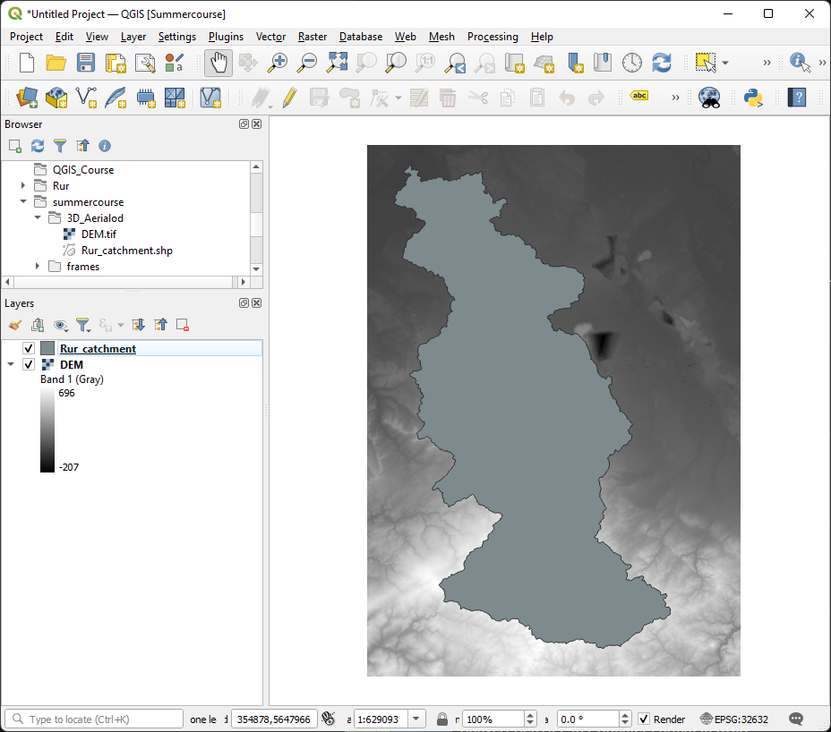
We'll first concentrate on the DEM and derive the flow direction that we need as an input to calculate the distance to the rivers.
4. Hide the Rur_catchment layer by unchecking its box in the Layers panel.
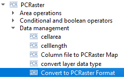
5. In the Processing Toolbox go to PCRaster | Data management | Convert to PCRaster Format.
6. In the Convert to PCRaster Format dialog choose DEM as Raster layer, Scalar for the Output data type (it's continuous data!) and save the result in the folder of the tutorial data with the name dem.map.
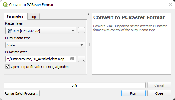
7. Click Run to convert the layer. Click Close to close the dialog.
Now we can calculate the flow direction layer (or LDD).
8. In the Processing Toolbox go to PCRaster | Hydrological and material transport operations | lddcreate.
9. In the Lddcreate dialog choose dem as DEM layer and keep the other parameters as default. Save the result as flowdirection.map in the folder with the data for this tutorial.
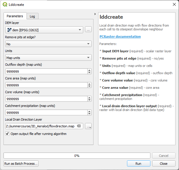
10. Click Run. This can take a few minutes. After processing click Close to close the dialog.
Now we have our flow direction layer we can derive the streams.
3. Derive Streams
In this section we're going to derive the streams. You can calibrate Strahler orders or flow accumulation.
Here we'll use the Strahler orders larger than or equal to 8.
1. In the Processing Toolbox go to PCRaster | Hydrological and material transport operations | streamorder.
2. In the Streamorder dialog choose flowdirection as the Local Drain Direction layer and save the result as strahler.map.
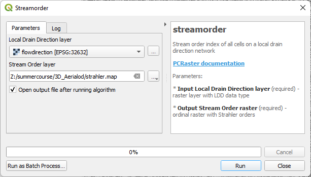
3. Click Run. Click Close after processing.
4. Open the Layer Styling panel by clicking . Style the result using the Paletted/Unique values renderer and a blue ramp. We use this renderer, because Strahler orders are ordinal.
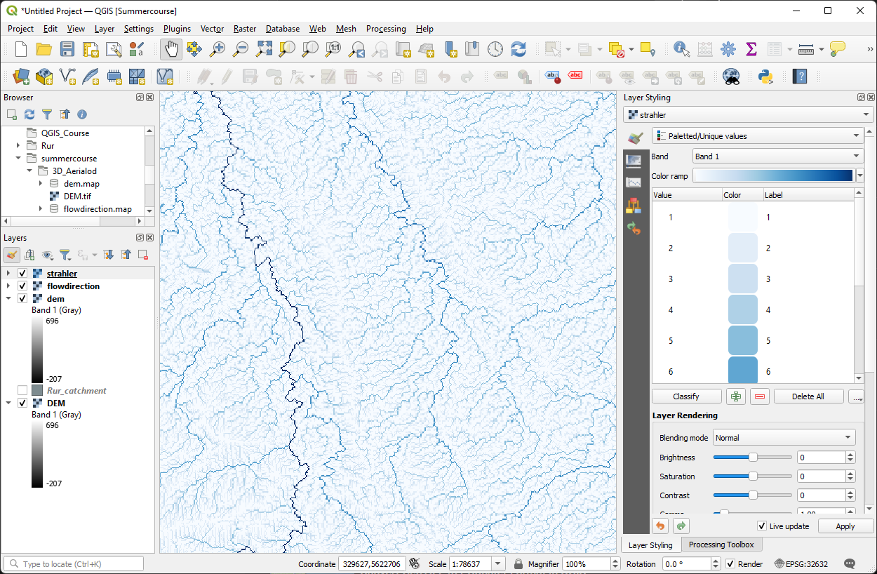
We'll consider Strahler orders larger than or equal to 8 as the rivers. In the next steps we'll create a boolean layer with the rivers.
First we'll create an ordinal raster with value 8 for each cell. Ordinal, because the Strahler order raster has the ordinal data type.
5. In the Processing Toolbox go to PCRaster | Data management | Spatial.
6. In the Spatial dialog type value 8 as Input nonspatial, choose Ordinal as Output data type and choose any of the PCRaster layers as Mask layer (all PCRaster layers that we have created have the same dimensions. Save the result as ordinal8.map.
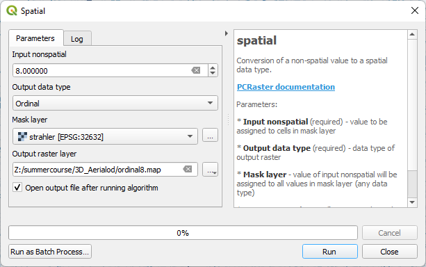
7. Click Run. Click Close to close the dialog after processing.
Now we can calculate the boolean river layer with True for cells >= 8 and False for the other cells.
8. In the Processing Toolbox go to PCRaster | Conditional and boolean operators | comparison operators.
9. In the Comparison Operators dialog choose strahler as Input raster, >= as Comparison operator and ordinal8 as the second Input raster. Save the result as rivers.map.
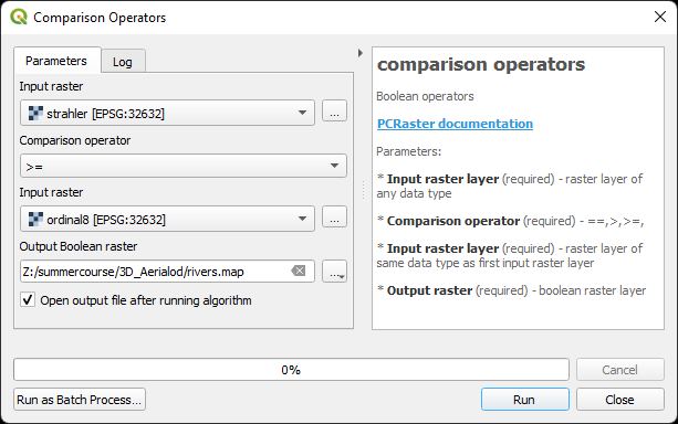
10. Click Run. Click Close after processing.
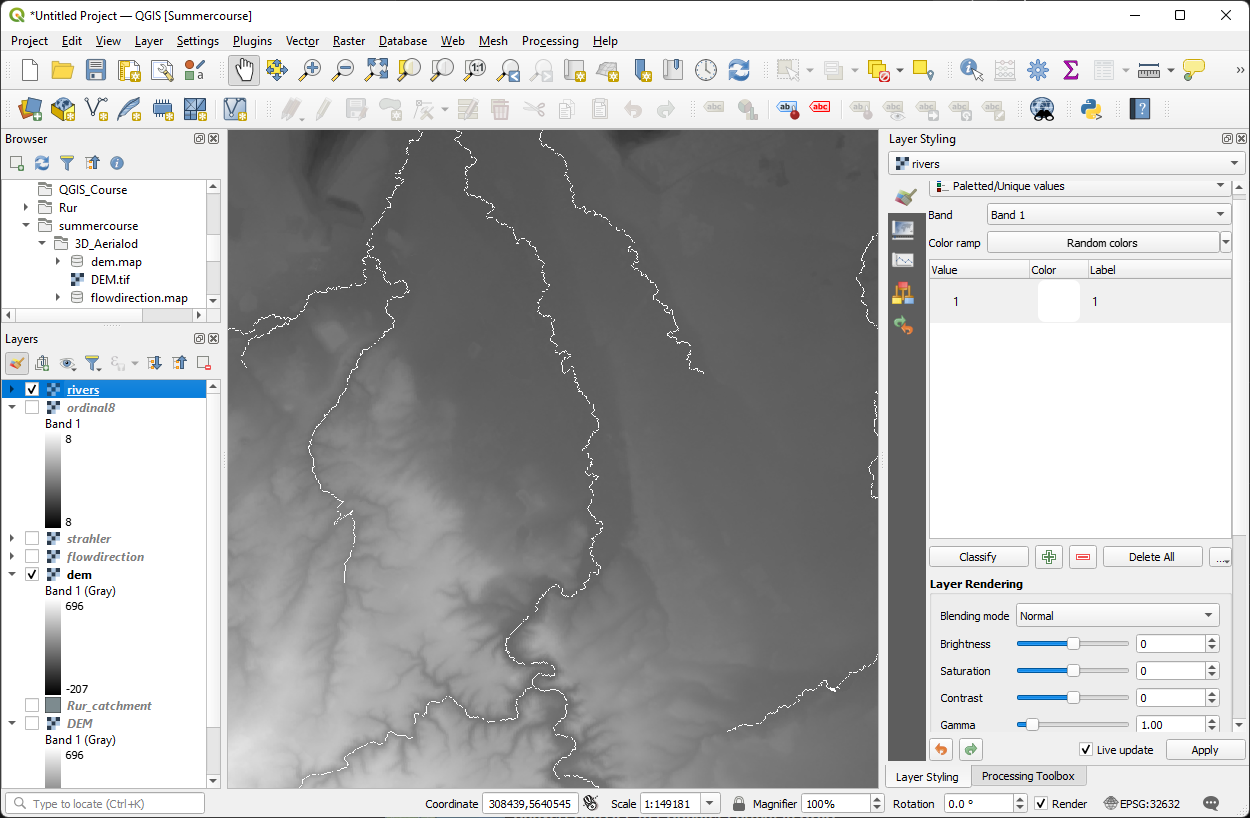
We want the rivers to be white and the other cells to be transparent.
11. Go to the Layer Styling panel and make sure rivers is the target layer.
12. Select the Paletted/Unique values renderer, because rivers is a boolean layer.
13. Click Classify.
14. Select the 0 row and click  to remove it. Then the zero's will be transparent.
15. Change the color of the ones to white.
16. Check the result by only showing the rivers over the dem layer.
Now we're ready to calculate the distances to the river.
4. Calculate Distance to River
In this section we'll calculate the distance to the river cells. We'll not calculate the Euclidean distance, but the distance over the flow direction, which is more realistic for runoff.
We'll use the ldddist tool from the PCRaster Tools plugin. This tool needs a friction layer. We'll create a friction layer with cells that have a value of 1. In that way the calculated distances are in map units.
1. In the Processing Toolbox go to PCRaster | Data management | spatial.
2. In the Spatial dialog type value 1 for the Input nonspatial. Choose Scalar for Output data type, because the friction layer should be in the scalar data type. For the Mask layer choose again any of the PCRaster layers. Save the result to friction.map.
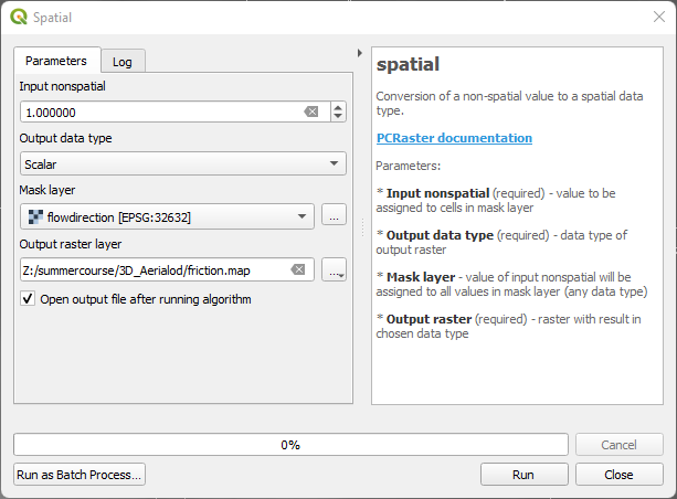
3. Click Run. Click Close after processing.
Now we can calculate the distance to the rivers.
4. In the Processing Toolbox go to PCRaster | Hydrological and material transport operations | ldddist.
5. In the Ldddist dialog choose flowdirection as LDD layer, rivers for Cells to which distance is calculated (Boolean), friction for the Friction layer and save the result as distance.map.
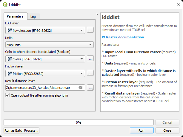
6. Click Run. Click Close after processing.
Now we have for each cell the distance to the river in meters visualized in grayscale.
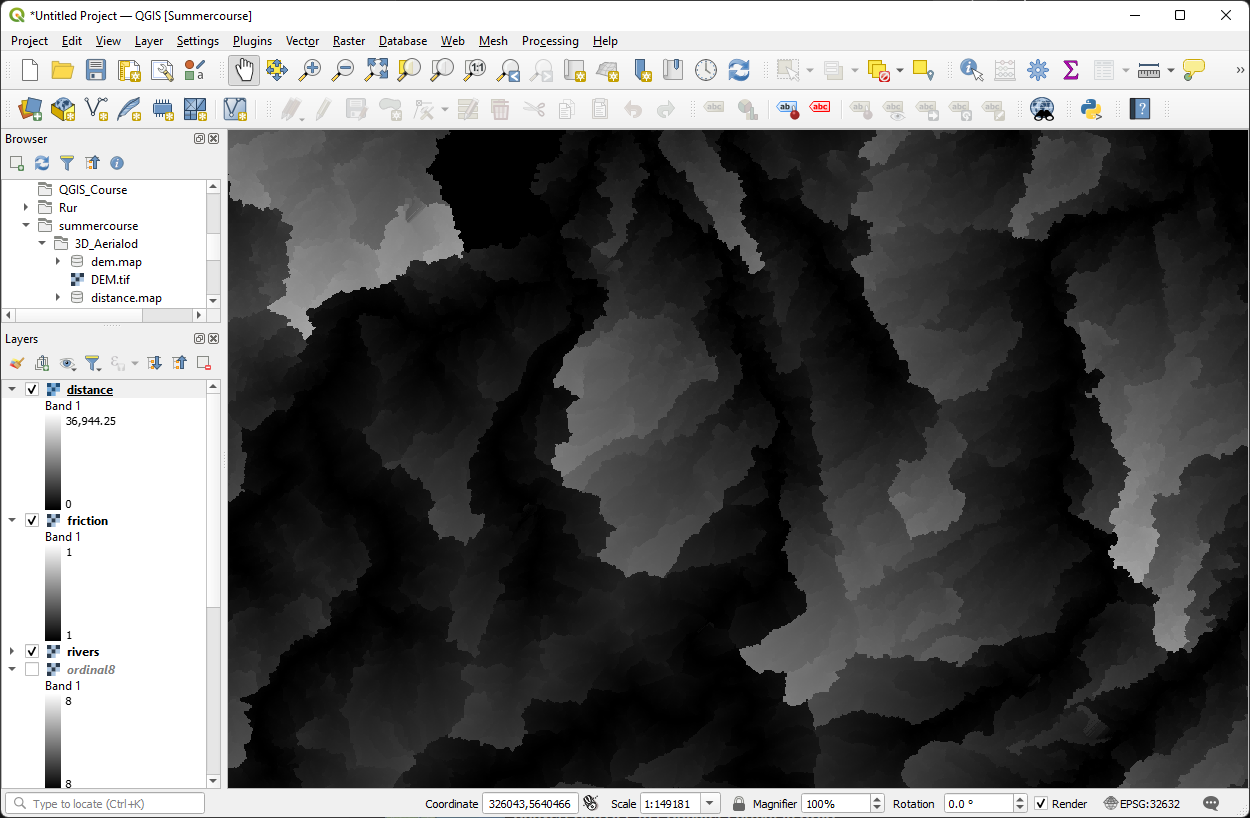
In the next section we'll finalize the inputs for Aerialod.
5. Finalize the Styling
In the next section we'll visualize our result in 3D using Aerialod. Aerialod expects a grayscale png file where black is low and white is high.
Let's style our map in such a way that it shows nicely in Aerialod.
1. Reorder the layers in such a way that the Rur_catchment polygon is on top, followed by the rivers layer and at the bottom the distance layer. Hide all other layers.
We're only interested in the area inside the catchment boundary, so we're going to create a black mask for the outside area, because black will result in the lowest height in Aerialod.
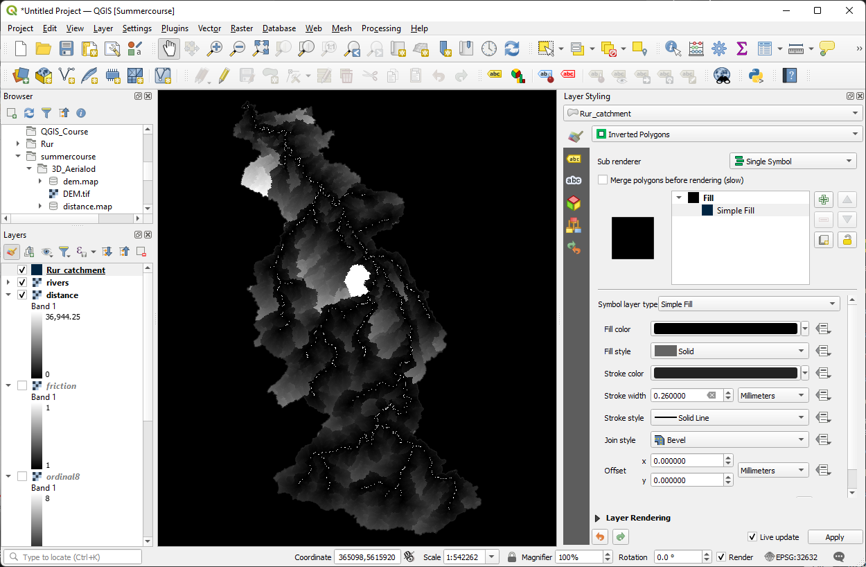
2. Go to the Layer Styling panel and make sure that Rur_catchment is the target layer.
3. Change the Single Symbol renderer to Inverted Polygons.
4. Click on Simple Fill and change the Fill color to black.
It would be good for the user to see some places as a reference. We can add some places from OpenStreetMap using the QuickOSM plugin.
5. Make sure you've installed the QuickOSM plugin from the plugins manager and click  to open the dialog.
6. Use Key=place and Value = city. Make sure that you only download the cities for the Canvas Extent and that you choose Points.
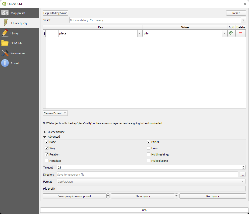
7. Click Run query and close the dialog when it's done.
Now the cities have a random color. To make them stand out in the 3D map, we need to make them white.
Also note that the city layer is a temporary scratch layer indicated with the  icon. Let's make it permanent before we continue.
8. Click on  and save the scratch layer as cities.shp.
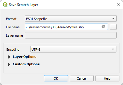
9. Click OK.
Now the is gone and we know that the layer is saved.
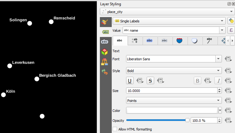
10. Go to the Layer Styling panel and make sure that the place_city layer is the target layer.
11. Choose the dot white symbol.
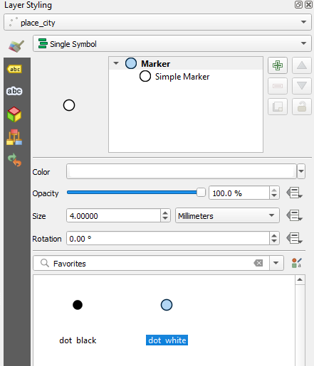
12. Click on Simple Marker and change the Stroke style to No Pen to remove the outline that we don't need.
Besides the dots we also want to show the names of the cities. We'll also make them white so they pop out of the 3D map.
13. In the Layer Styling panel go to the Label  tab .
tab .
14. Choose Single Labels and for Value choose the Name field.
15. Go to the Font  tab and choose Liberation Sans with Style Bold.
6. Creating the Print Layout
The
user also needs a legend to understand which height in 3D corresponds
with which distance. A north arrow is also important in 3D, because it's
harder to orient. We can finalize the map with these items in the Print Layout.
1. In the main menu go to Project | New Print Layout.

2. Call the new Print Layout Aerialod and click OK.

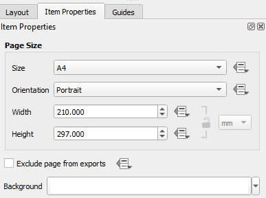
First we need to change the sheet from landscape to portrait given the orientation of our catchment.
3. Right-click on the page and choose Page Properties... from the context menu.
4. In the Item Properties change Orientation to Portrait.
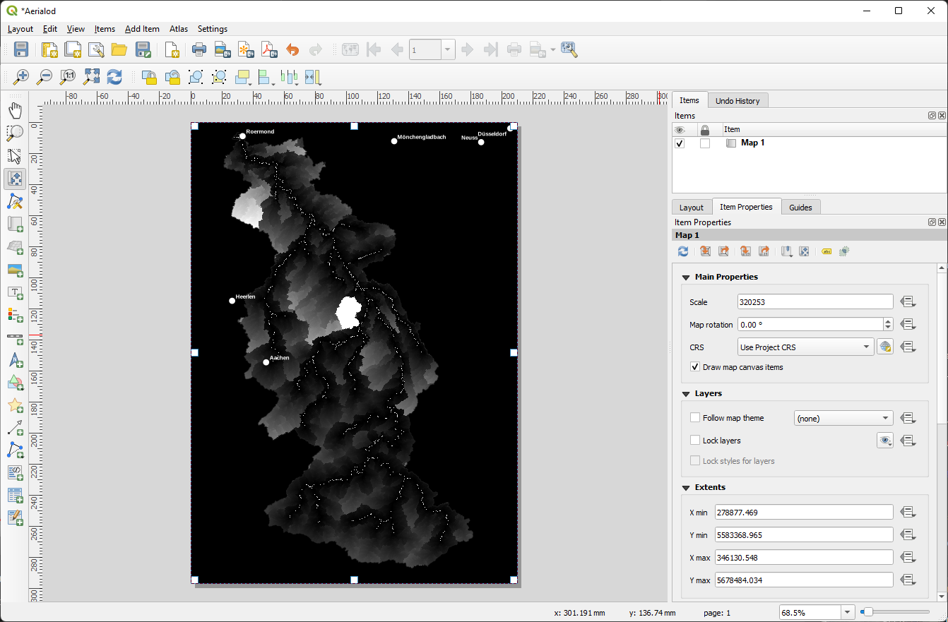
Now we can add the map.
5. Click the Add map  icon and drag a rectangle that covers the complete sheet. Note that the handles snap to the corners of the sheet.
6. Use the Move item content  tool in combination with the mouse scroll wheel to adjust the position and scale of the map. With Ctrl-Scroll you can make small steps when you want to zoom in or out.
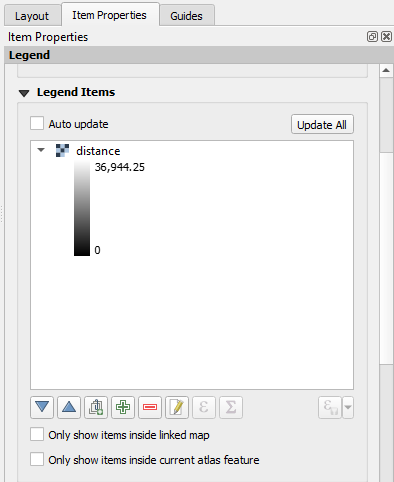
Now let's add a legend.
7. Click the Add legend icon and drag a box where there's space outside of the catchment area.
8. In the Item properties uncheck Auto update.
9. We only need the distance legend, so select all other items and use the  button to remove them.
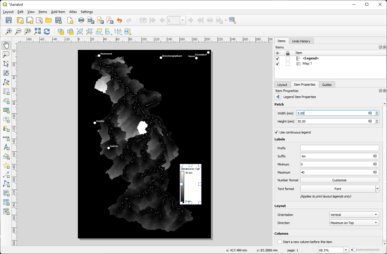
10. Double-click on the distance text and change the text to Distance to river.
11. Remove the Band 1 item by selecting it and clicking the button.
It's better to show the distance in km than in m. Let's change that.
12. Double-click on the ramp and type km at Suffix. Don't forget to type a space before the unit.
It's not possible to calculate the min/max values automatically as kilometers, so we need to type the min/max values.
13. Change the Minimum to 0 and the Maximum to 40 (a round number, the details are not visible anyways).
14. Change the Width to 5 and the Height to 50 mm.
15. Click  to go back.
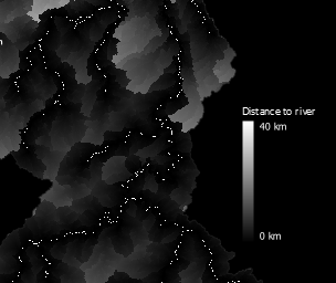
The legend needs a few more tweaks.
16. Uncheck the box before Background to make it transparent.
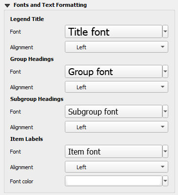
Now the black fonts are not readable.
17. Expand the Fonts and Text Formatting section by clicking the black arrow.
18. Change the Font color to white.
Now the legend looks like this:
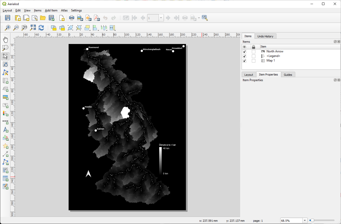
Let's add the north arrow.
19. Click the Add North Arrow icon and drag a rectangle in a black space outside of the catchment where you want to place it.
We'll use the simple default north arrow. Don't make it too big!
On 3D maps we can't use the 2D scale bar, because of the perspective. So we're ready to export the map to a png file.
20. Click the Export as image icon. Give it an output file name and make sure to choose the PNG format.
21. In the Image Export Options keep the defaults and click Save.
When you have successfully exported our grayscale map, we're going to make it visually attractive in Aerialod. Save the project and close QGIS before you continue.
7. Install and Use Aerialod
We're going to use Aerialod for creating the 3D map. It's free software that is easy to install.
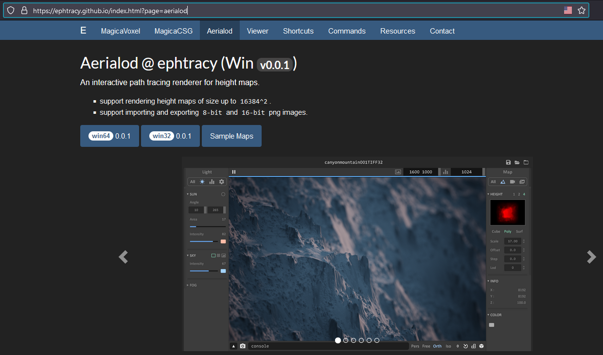
1. Go to the website of Aerialod.
2. Download the zip file. You probably need the 64 bit version (win64).
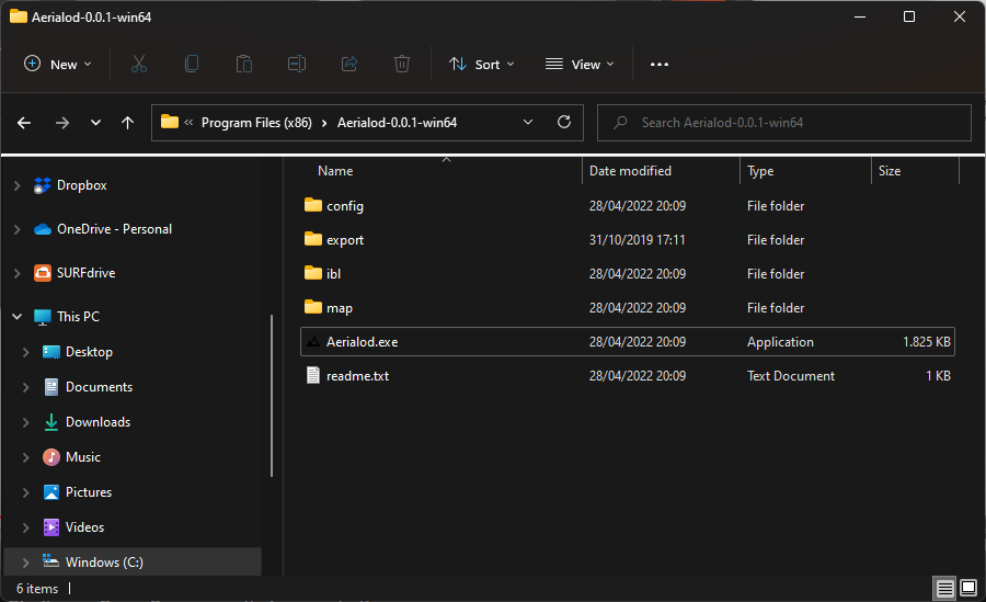
3. Extract the contents of the zipfile somewhere on your hard drive, e.g. C:\Program Files.
4. Double-click on Aerialod.exe to run the program.
5. Maximize the window.
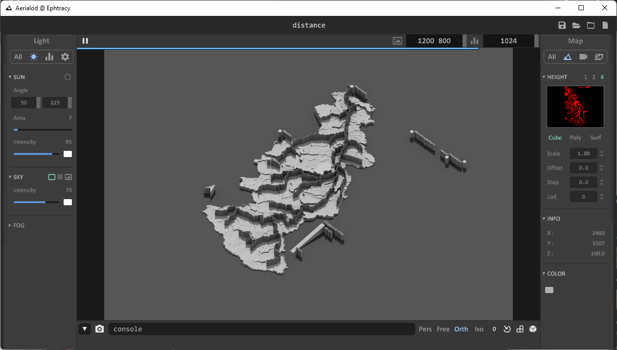
6. Click the Open Map  icon in the upper left and open the PNG file that you saved in the QGIS Print Layout.
It will start rendering immediately. The blue bar shows how far it is with rendering. It will only render when the window has focus and it will start re-rendering when you change settings.
7. Use the scroll wheel and right mouse button to respectively zoom and rotate.
Explore the different settings by yourself. Change the color to a light blue.
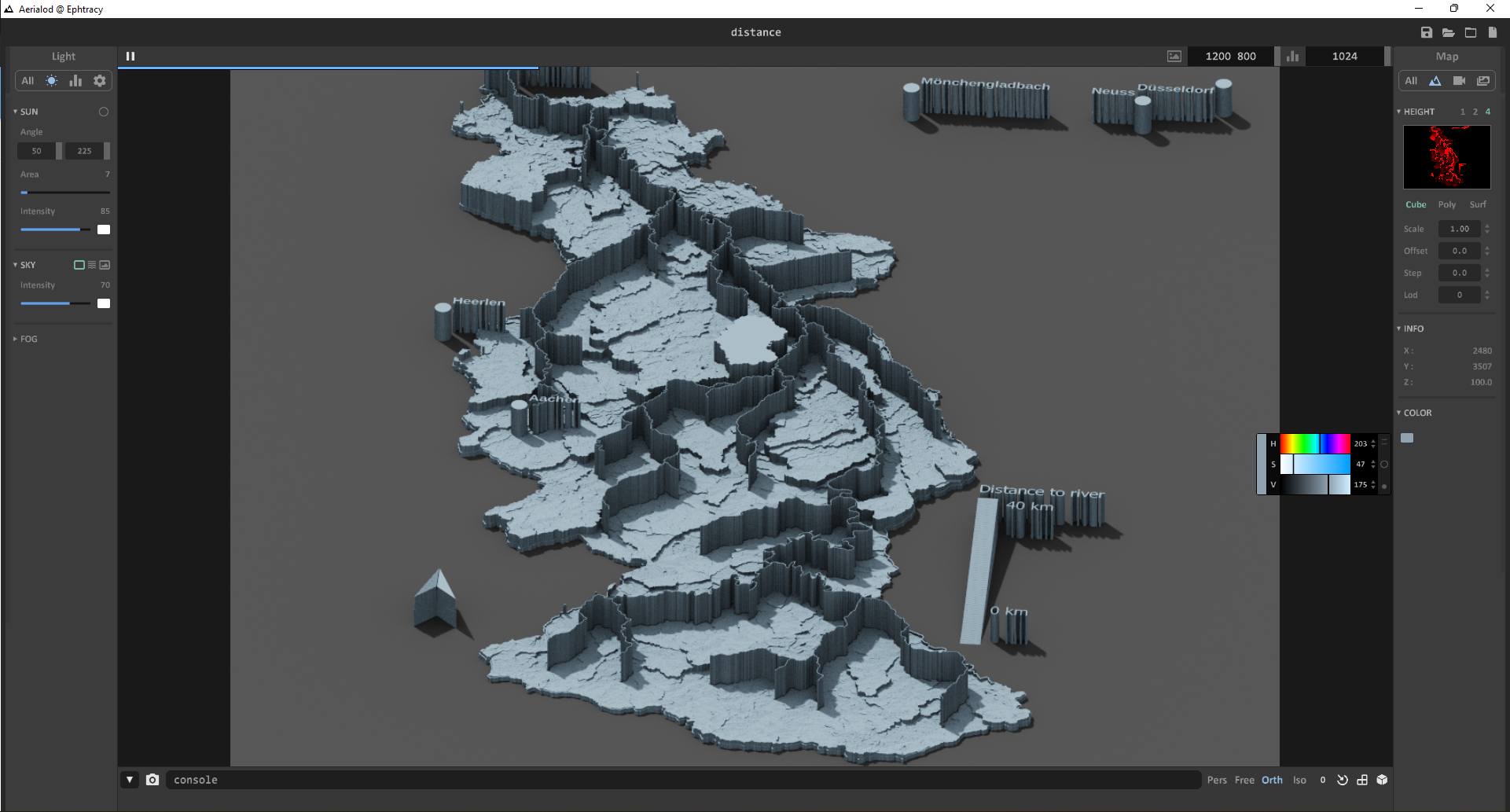
8. When you have found a nice position, save a snapshot by clicking  in the lower left.
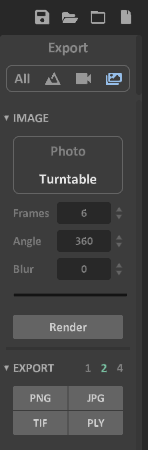
You can also save an animation of a rotating scene. You can explore the settings here. Note that it takes hours to render a large scene at hight quality.
8. Conclusion
In this tutorial you've learned how to create 2.5 D visualisations in Aerialod.
Watch this video for the steps: