Tutorial: Create and Use Virtual Point Clouds (VPC)
| Site: | OpenCourseWare for GIS |
| Course: | Point cloud processing with QGIS and PDAL wrench |
| Book: | Tutorial: Create and Use Virtual Point Clouds (VPC) |
| Printed by: | Guest user |
| Date: | Wednesday, 29 July 2026, 4:13 AM |
1. Introduction
Point cloud data is often provided in tiles. After downloading the tiles you need to merge them for further analysis. With virtual point clouds, you don't need to physically merge the tiles, which reduces the amount of disk space needed for intermediate results.
A virtual point cloud (VPC) is a new method to handle a large number of point cloud files. It is a file format that references other point cloud files, similar to the concept of virtual rasters. At its core, a VPC file is a simple JSON file with a .vpc extension, containing references to actual data files (e.g. LAS/LAZ or COPC files) and additional metadata extracted from the files. Tools supporting virtual point clouds handles the whole tiled dataset as a single data source. This makes it easier to display and analyse all the point cloud files listed in the virtual file.
In this tutorial you'll learn to:
- Download AHN4 point cloud tiles from Geotiles.nl
- Check point cloud information
- Build a virtual point cloud layer from tiles
- Visualise the result in the QGIS 3D view
2. Download AHN4 tiles
In this workshop we're using AHN4 point cloud tiles of the Netherlands, that can be downloaded from Geotiles.nl. Feel free to use your own LAZ data. For Estonia, data is available here.
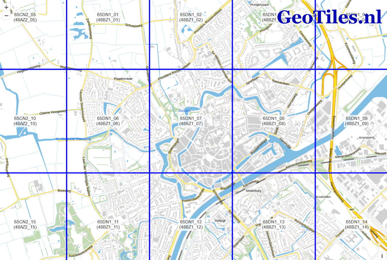
1. In a web browser go to Geotiles.nl
2. Download the tiles of a city of your choice, by zooming in until you see the subtiles. Save the tiles in a dedicated folder on your hard drive.
In this workshop we'll use Middelburg as an example. For the historic center of Middelburg you can download the following tiles:
- 65DN1_07.LAZ
- 65DN1_08.LAZ
- 65DN1_12.LAZ
- 65DN1_13.LAZ
3. Load point cloud tiles in QGIS
In this chapter we'll load the downloaded point cloud tiles in QGIS.
1. Start QGIS Desktop. Make sure you use version 3.32 or newer.
2. Locate the folder with your downloaded tiles in the Browser panel. Right-click on the folder name and choose Add as a Favorite from the context menu.
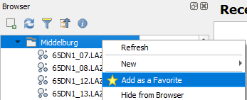
Now we have created a shortcut in the Browser panel, where we can find the files.
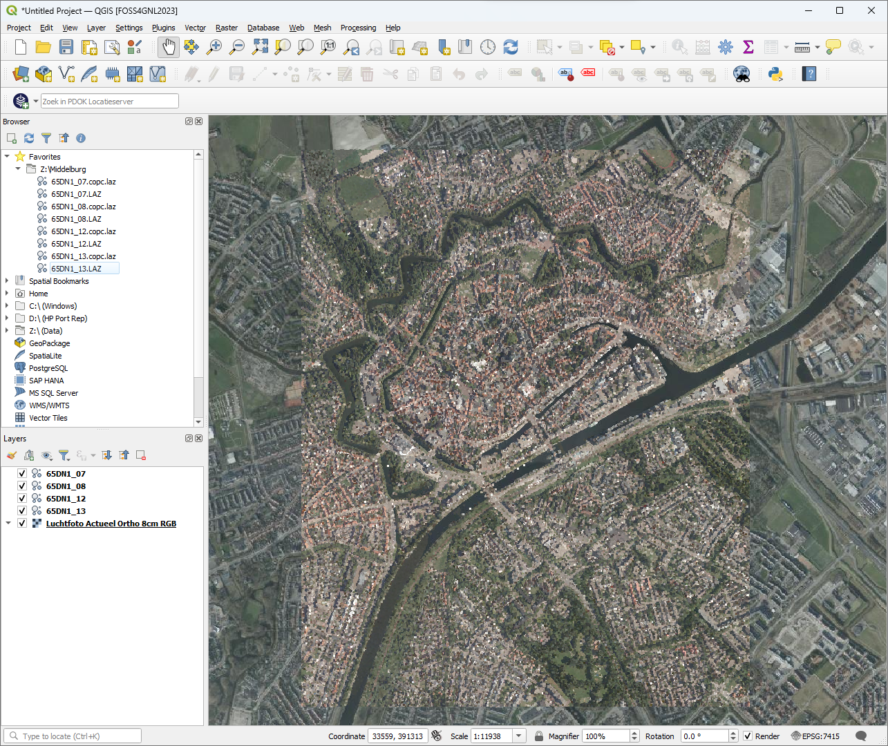
3. Select the .LAZ files and drag them from the Browser panel to the map canvas.
QGIS will now show the extent of the tiles with a dashed red border and will automatically convert the LAZ files to the Cloud Optimized Point Cloud (COPC) format. This can take some time.

After the conversion has finished, you'll see the RGB coloured points in the map canvas and you'll find the .copc files in the Browser panel.
Let's check if the point cloud is correctly georeferenced. We'll do that by adding an aerial photograph from the PDOK Services plugin.
4. In the main menu, go to Plugins | Manage and Install Plugins....
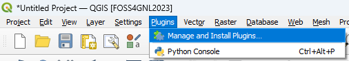
5. In the Plugins Manager dialog search for PDOK Services plugin.
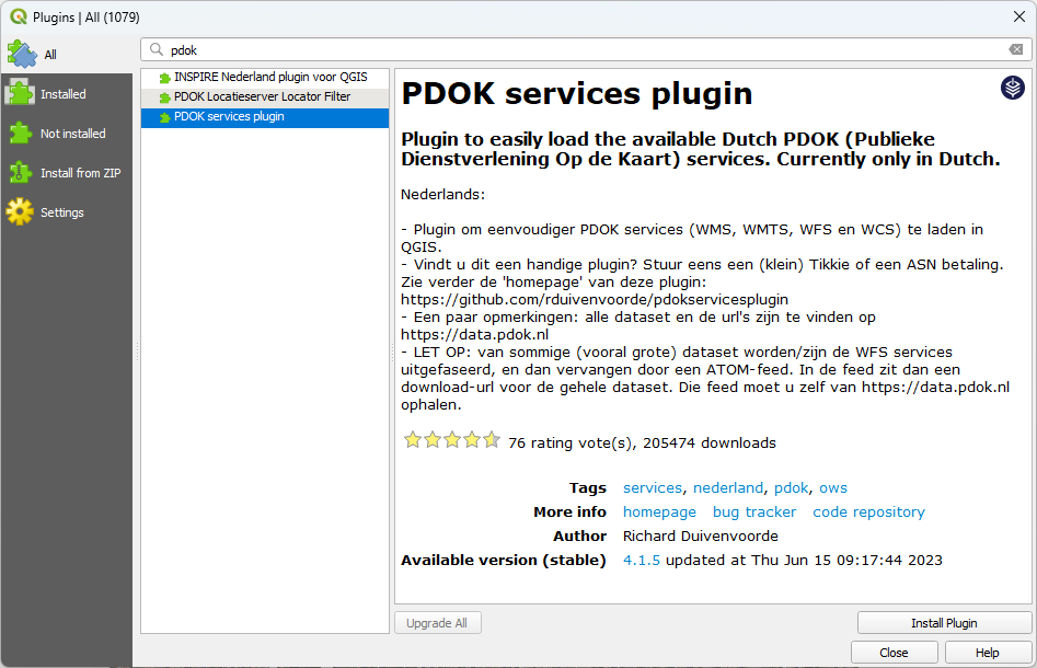
6. Click Install Plugin.
7. Click Close to close the dialog after successfully installing the plugin.
8. In the toolbar, look for the PDOK Services Plugin icon  and click it.
9. In the PDOK Services Plugin dialog select the first layer: Luchtfoto Actueel Ortho 8cm RGB, which is a high resolution aerial photograph provides as WMTS layer.
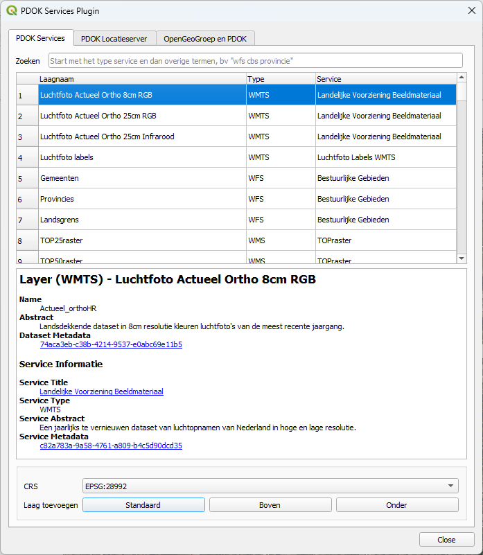
10. Click the Onder button to add the layer below the LAZ files.
11. Click Close to close the PDOK Services Plugin dialog.
You can see in the map canvas that the point cloud data fits nicely with the aerial photograph.
In the next section, we'll check the properties of the point cloud tiles.
4. Check point cloud information
Now we can check what projection and attributes are provided with the point cloud data.
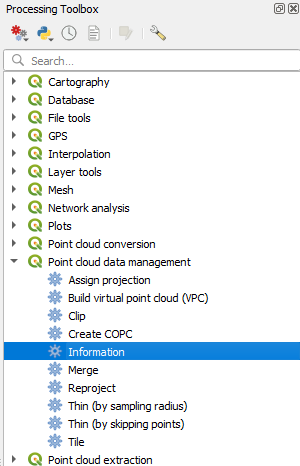
1. Click the Toolbox icon  in the main toolbar to open the Processing Toolbox panel.
2. In the Processing Toolbox expand Point Cloud Data Management by clicking the arrow and double-click on the Information tool.
3. In the Information dialog, select one of the point cloud tiles and use the Browse  button to browse to the location where you want to save the resulting HTML file.
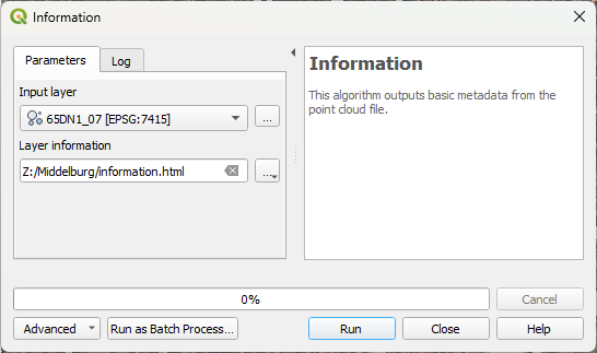
4. Click Run.
The result can be found in:
- The Log tab of the Information dialog window.
- In the Results Viewer panel by double clicking on Layer information.
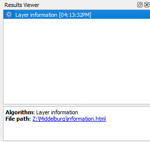
- In the HTML file that was saved.
5. Check the result and close the dialog. Also close the Results Viewer panel.
- How many points are in the tile?
- What is the projection?
- Which attributes are present?
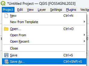
Save the project before we continue.
6. In the main menu, go to Project | Save As... and save the project in the folder with the LAZ files with a name of your choice, e.g. Middelburg.qgz.
In the next section, we're going to merge the tiles in a Virtual Point Cloud layer.
5. Build a Virtual Point Cloud layer
Our point cloud data is still divided in tiles. For further processing we need to merge them into one layer. We could do that with the Merge tool, which will create a large LAZ or COPC layer. Here, however, we're going to create a Virtual Point Cloud (VPC) layer. The advantage is that we're not copying the data, but can use the VPC layer in algorithms that we need for further analysis.
The Build virtual point cloud (VPC) tool works with the LAZ files, but will only show the boundaries. It will work with further processing. However, if we want to see the RGB colours or other attributes, we need to use the COPC format.
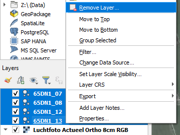
1. In the Layers panel, select all LAZ layers and right click on the selection. Then choose Remove Layer from the context menu. In the popup, click OK to confirm.
Now you'll only have the aerial photograph.
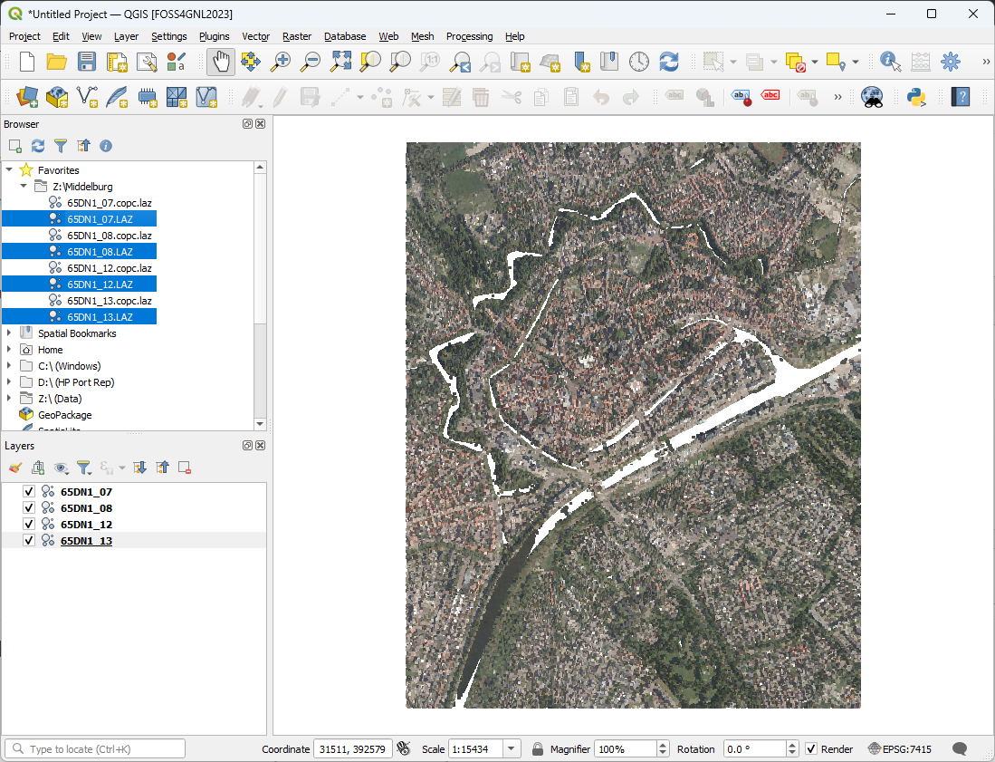
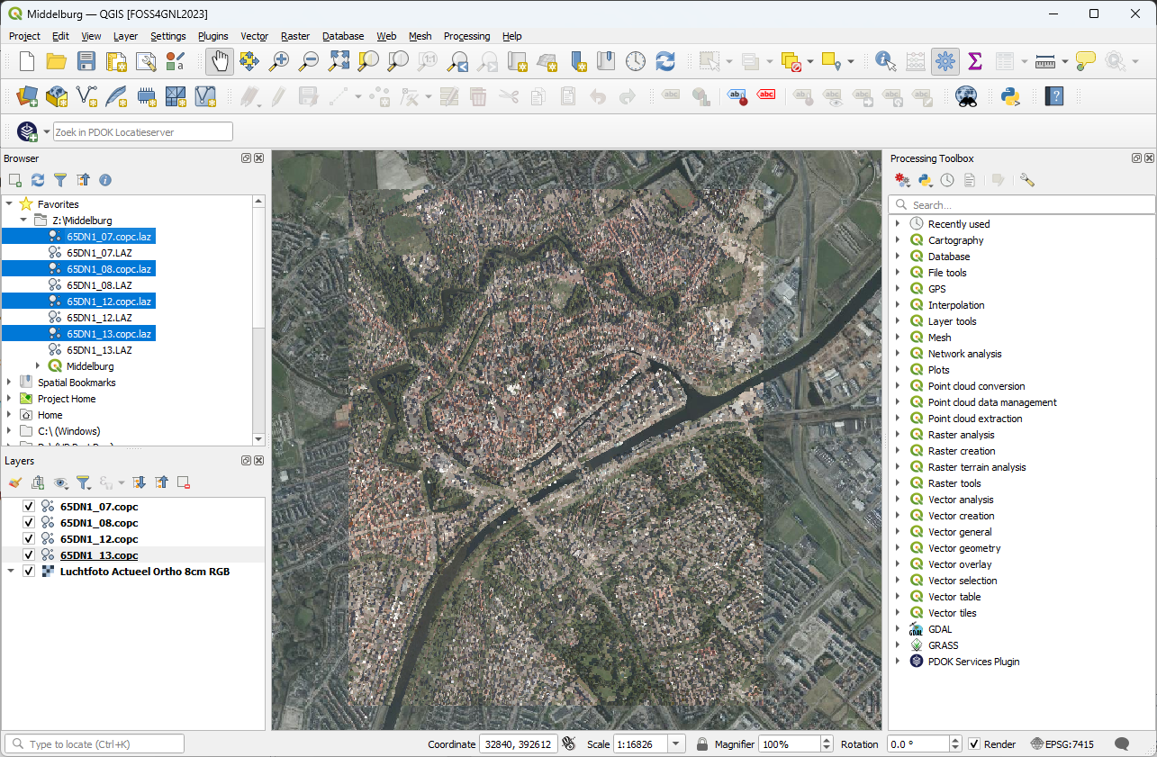
2. In the Browser panel, select the COPC layers with the CTRL-button pressed and drag them to the map canvas.
3. Save the project by clicking  .
.
Your screen now looks like this:
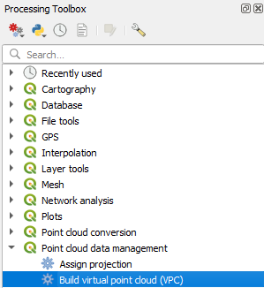
4. In the Processing Toolbox go to Point cloud data management | Build virtual point cloud (VPC).
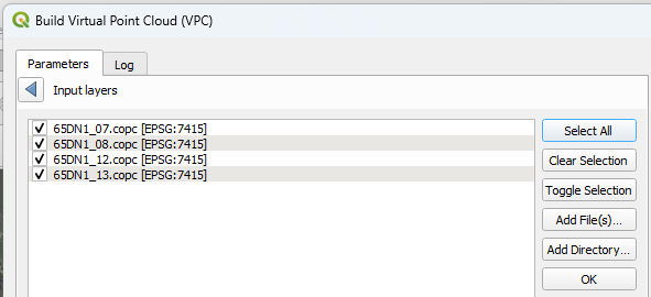
5. In the Build Virtual Point Cloud (VPC) dialog, click the Browse  button at Input layers.
6. Click Select All and OK.
7. Now check the boxes to Calculate boundary polygons, Calculate statistics and Build overview point cloud. The boundary polygons will only cover the areas with data points, so they'll not necessarily be rectangular as with the extent. To calculate statistics is useful for visualisation and processing. The overview point cloud is comparable with pyramid layers for rasters and helps with efficiently visualising the point cloud data at different zoom levels.
8. Save the result in the folder of the project with a filename with the extension .vpc (make sure you choose that extension in the Save file dialog).
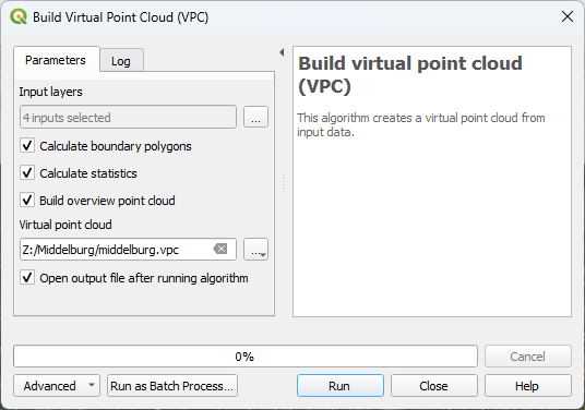
9. Click Run. Click Close to close the dialog after processing.
10. Remove the individual point cloud tiles from the Layers panel (select them with the Ctrl-button pushed, right-click on the selection and choose Remove Layer from the context menu).
11. Hide the aerial photograph by unchecking the box before the layer name in the Layers panel.
Now your screen will look like this:
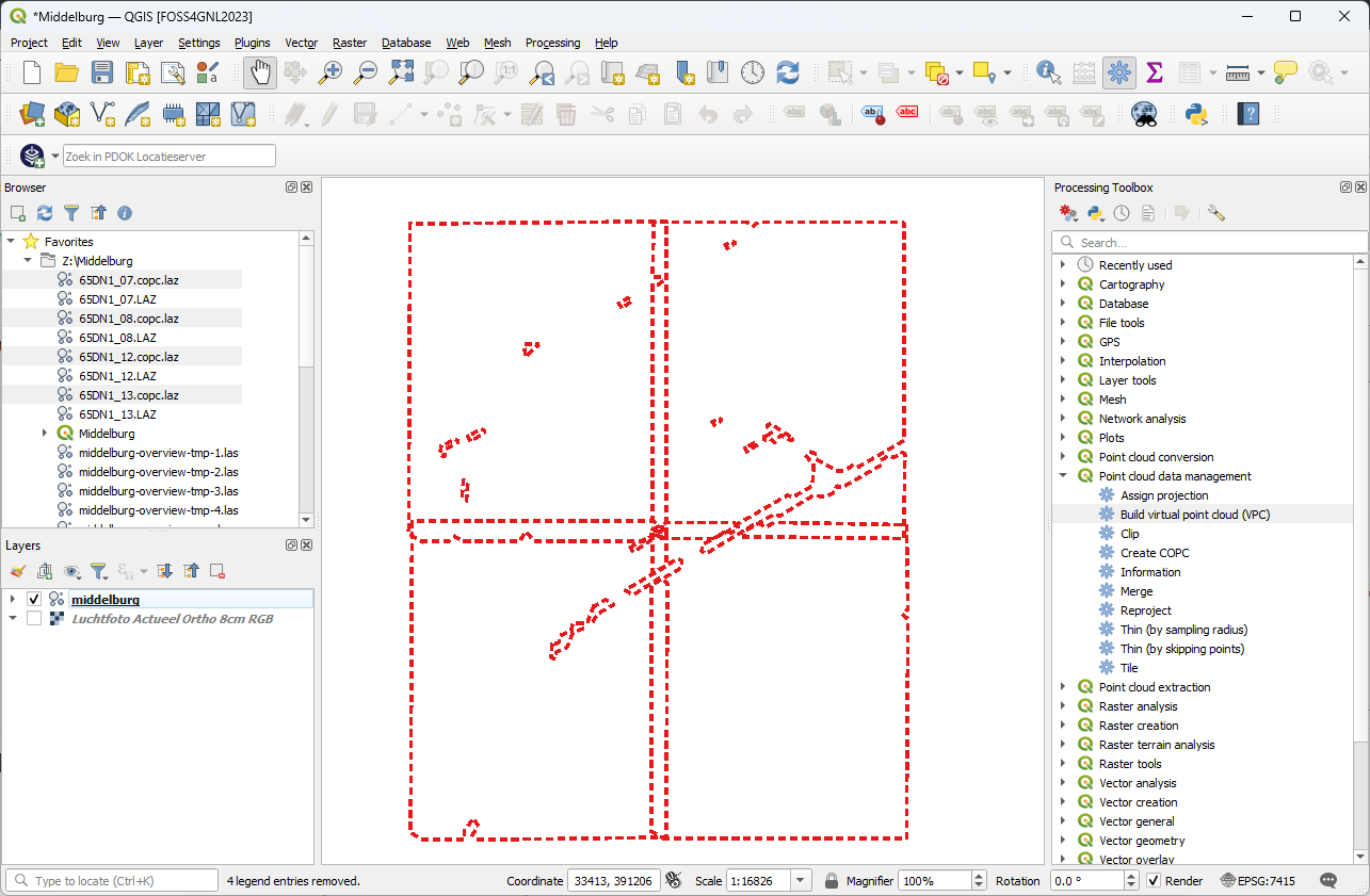
12. Zoom in on the map canvas.
You'll now see the points coloured with the classification attribute.
In the next chapter, we'll change the visualisation attribute and visualise the result in 2D and the 3D View.
6. Visualise point clouds in 2D and 3D
It's nicer to look at the RGB colours instead of the classification attribute. We can see the RGB colours again by changing some settings in the Layer Styling panel.
1. In the Layers panel, make sure that the VPC layer is selected and click  to open the Layer Styling panel.
2. In the Layer Styling panel, click on the Classification renderer and change it to RGB.
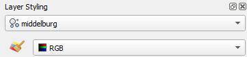
You were now changing settings in the 2D styling tab .
We can also visualise point cloud layers in the 3D View.
You can change the settings for the styling in the 3D View in the 3D View  tab of the Layer Styling panel. By default it is set to Follow 2D symbology, which is okay for our purpose.
Now we're ready to visualise the point cloud in the 3D View.
3. To fill in the voids (missing points), unhide the aerial photograph layer by checking its box in the Layers panel.
4. In the main menu, select View | 3D Map Views | New 3D Map View.
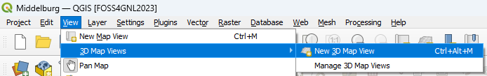
This will load a new window for the 3D view and starts rendering the point cloud layer.
By default the window will dock like other QGIS panels. However, often it's nicer to have the 3D view full screen.
5. In the 3D Map 1 window, click the  to undock the window.
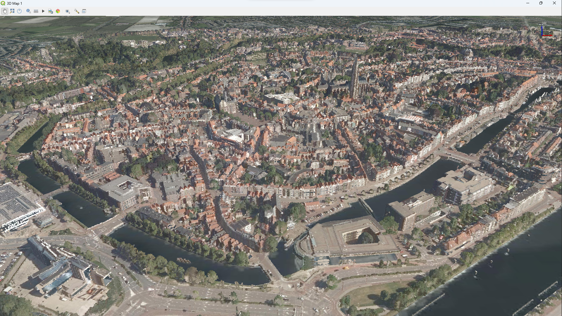
6. Maximize the 3D Map 1 window.
Now you can navigate in the 3D view. You can use the compass panel on the right side of the window or try to use the mouse. Dragging the scroll wheel will tilt the scene. By dragging the left button, you can pan in all directions. By dragging the right button you can zoom in/out. If you don't need the compass, you can click  to hide the panel.
- Try to visualise other attributes in 2D and 3D by changing settings in the Layer Styling panel.
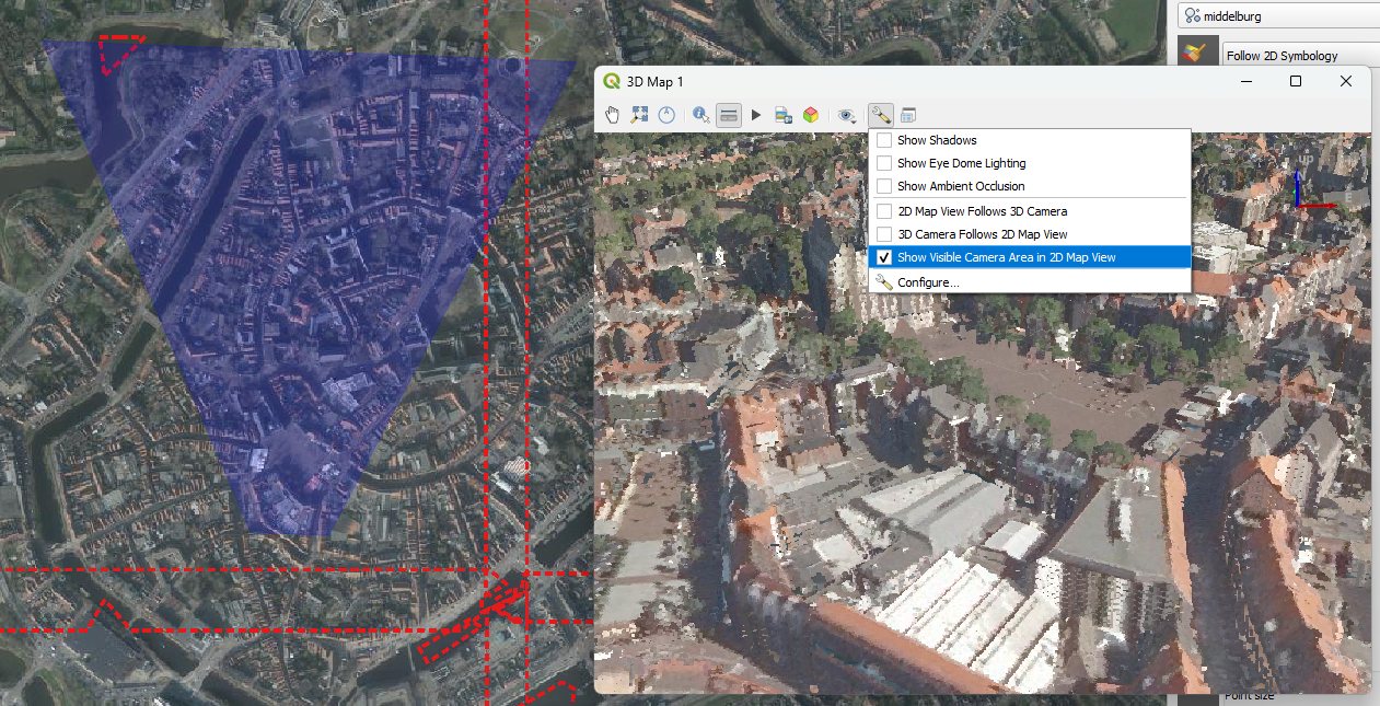
- Use the
 tool to measure heights of buildings.
 - Play with the
 options to visualise in the 2D map, which area is shown in the 3D View.