Tutorial: Interpolate Point Clouds to Rasters
| Site: | OpenCourseWare for GIS |
| Course: | Point cloud processing with QGIS and PDAL wrench |
| Book: | Tutorial: Interpolate Point Clouds to Rasters |
| Printed by: | Guest user |
| Date: | Thursday, 25 June 2026, 8:18 AM |
1. Introduction
In this tutorial we're going to create a raster of the point cloud layer. First, we'll clip the area of interest. Next, we'll use the Inverse Distance Weighting (IDW) method to create rasters of different resolutions. Finally, we'll use the triangulation (TIN) method and compare the results. For comparison, we'll use two linked 2D views and elevation profiles.
After this tutorial, you're able to:
- clip point cloud data
- interpolate point cloud data with the Inverse Distance Weighting (IDW) method
- interpolate point cloud data with the triangulation (TIN) method
- compare rasters using two 2D views
- compare rasters using elevation profiles
We'll continue with the VPC layer of the previous tutorial. Alternatively, you can use any other point cloud tile.
2. Clip point cloud data
Let's first clip our point cloud layer to an area of interest. In this example, we'll digitize a polygon around the historic center of Middelburg and use that to clip the VPC layer of the previous tutorial.
1. Open QGIS Desktop with the project from the previous tutorial or load a point cloud layer into an empty project.
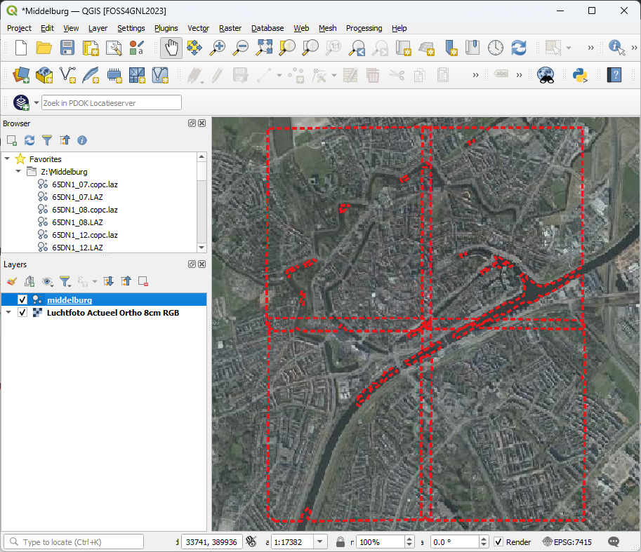
We'll show the aerial photograph in the background, because that's easy for digitizing our area of interest. Alternatively, you can use the OpenStreetMap layer that you can drag from the Browser panel, under XYZ layers, and drop it in the map canvas.
Because we only need a polygon to clip the point cloud layer and we'll not use it further, we're going to create a temporary scratch layer.
2. In the main toolbar, click  to create a temporary scratch layer.
3. In the New Temporary Scratch Layer dialog, type Area of interest as the Layer name, choose Polygon as the Geometry type and change the CRS to the project CRS, in this case EPSG:7415.
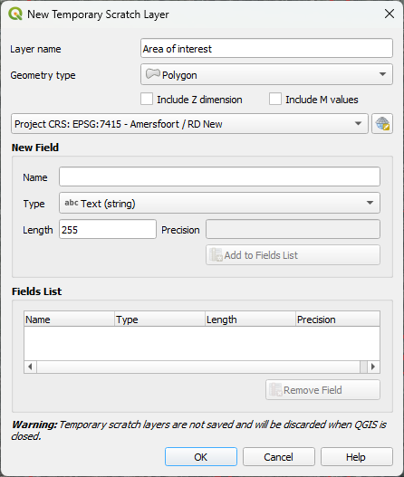
We don't need any attributes.
4. Click OK to create the empty polygon scratch layer.
The layer is automatically set to editing mode, so we can start digitizing the polygon.
5. Click  to add a polygon feature.
6. Digitize a polygon around your area of interest. In this example, we'll create a polygon for the historic center of Middelburg. With left-click you can add vertices, with backspace you can delete the last vertex and with right-click you close the polygon.
7. After digitizing the polygon, click  in the toolbar to toggle editing off and confirm that you want to save the edits.
Let's style the polygon with a white boundary without a fill colour.
8. In the Layers panel, click  to open the Layer Styling panel.
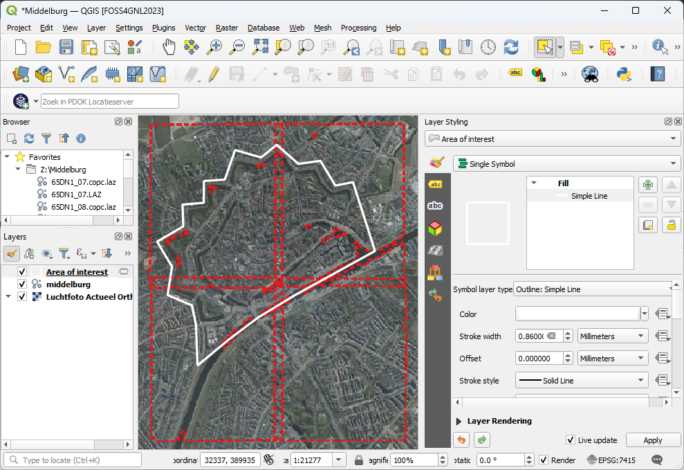
9. Make sure that the Area of interest layer is the active layer and click on Simple fill.
10. Change the Symbol layer type to Outline: Simple line.
11. Change the colour to white and the Stroke width to 0.86 mm.
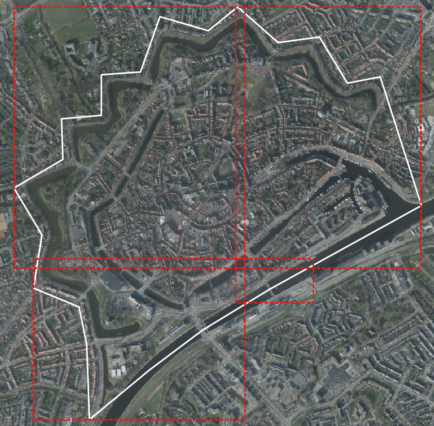
The result now looks like this:
Now we're ready to clip the point cloud layer with the digitized polygon.
12. Click  to open the Processing Toolbox panel.
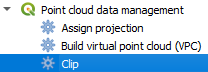
13. Go to the Point cloud data management | Clip tool.
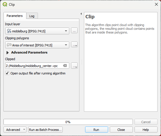
14. In the Clip dialog set the Input layer to the point cloud layer you want to clip, e.g. middelburg and choose Area of interest as the layer for Clipping polygons. Save the result in the VPC format, e.g. middelburg_center.vpc.
Note that until version 3.42, you can only save to the VPC format, because the input layer is in the VPC format! However, in 3.44.x it should be possible to save to COPC.
15. Click Run. Click Close after completion.
Note that you will only see the bounding boxes in red, because we're using the VPC format. If you hide the aerial photograph, you'll not see the RGB points. This is not a problem, because this is an intermediate result, before we start interpolating the points for our area of interest, which we'll do in the next chapter.
16. Save the Area of interest polygon by clicking  . We'll need the file later in the pdal wrench tutorial. Save it as boundary.shp.
3. Interpolate with IDW
In this chapter we're going to interpolate the point cloud data to raster using the Inverse Distance Weighting (IDW) method. IDW will assign elevations to unknown locations, based on a weighted average of the elevations of known points. The weights are determined by an exponential decay function with the distance to a known point.
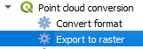
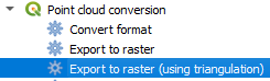
1. In the Processing Toolbox go to Point cloud conversion | Export to raster.
2. In the Export to Raster dialog, choose the clipped VPC layer (e.g. middelburg_center) as Input layer and the Z field as Attribute. Keep the Resolution of the density raster at 1 m and the Tile size for parallel runs at 1000 m. Save the result as DSM_IDW_1m.tif.
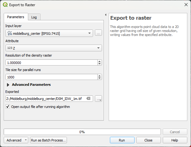
3. Click Run. Click Close after processing.
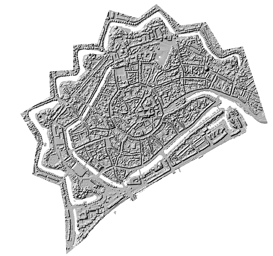
4. In the Layers panel, hide all layers except DSM_IDW_1m.
5. Go to the Layer Styling panel and change the renderer to Hillshade.
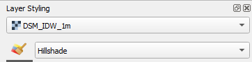
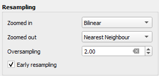
6. At the bottom of the Layer Styling panel change the Resampling Zoomed in to Bilinear and check the box for Early resampling.
7. Zoom in on the raster and check the result.
8. Repeat the same procedure for a Resolution of the density raster of 0.5 m , 0.25 m and 0.1 m. Save the output as DSM_IDW_05m.tif, DSM_IDW_025m.tif and DSM_IDW_01m.tif respectively.
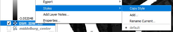
TIP: Click the history  icon in the Processing Toolbox and double-click last tool you've used today. Now you only have to change the Resolution of the density raster and the output file name. You can also copy the style of the 1 m result and paste it to the higher resolution results. Right-click on the layer and choose Styles in the context menu.
9. Compare the results by (un)hiding the layers. What do you see?
- Which resolution gives the best results?
Next, we'll use this resolution for another interpolation method.
4. Interpolate with TIN
In this chapter we're going to apply another interpolation method: Triangulated Irregular Network (TIN). It is a method of representing a continuous surface, such as terrain, using a network of non-overlapping triangles. The vertices of these triangles are the points in the point cloud. The triangles are then interpolated to a raster.
1. In the Processing Toolbox panel go to Point cloud conversion | Export to raster (using triangulation).
2. Choose the point cloud as the Input layer, e.g. middelburg_center. Change the Resolution of the density raster to 0.5 m. Keep the Tile size for parallel runs at 1000 m. Note that you don't need to select the Z field as attribute. This will be automatically used. Use DSM_TIN05m.tif as output file name.
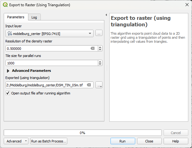
3. Click Run. Click Close after processing.
Note that this interpolation method is slower than IDW. On my computer it took 6 minutes.
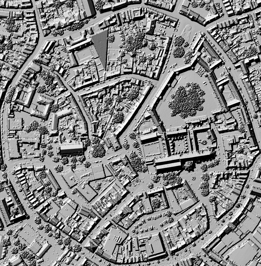
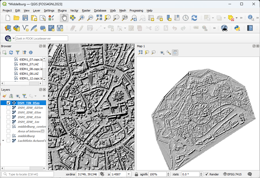
4. Inspect the result.
In the next chapter, we'll compare the results.
5. Compare the results
In this chapter we'll compare the results of the interpolations.
First we'll create map themes. Next, we'll visualise interpolation next to each other in two linked 2D Map Views. Finally, we'll use the Elevation Profile tool.
5.1. Create map themes
In QGIS, a Map Theme is a way to save the current visibility and style of layers in your project so that you can quickly switch between different layer configurations. This is useful when working with many layers and you want to focus on specific layers or combinations of layers at different times.
Let's create two map themes. One showing IDW and the other showing the TIN interpolation result.
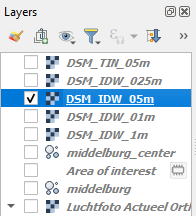
1. In the Layers panel, hide all layers, except DSM_IDW_05m.
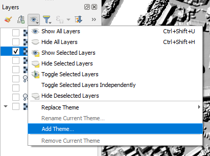
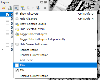
2. Click on the Manage Map Themes  icon and choose Add Theme... from the menu.
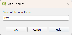
3. In the popup type IDW for the Name of the new theme and click OK.
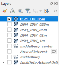
4. Now hide the DSM_IDW_05m layer and unhide the DSM_TIN_05m layer.
5. Click on the Manage Map Themes icon and choose Add Theme... from the menu.
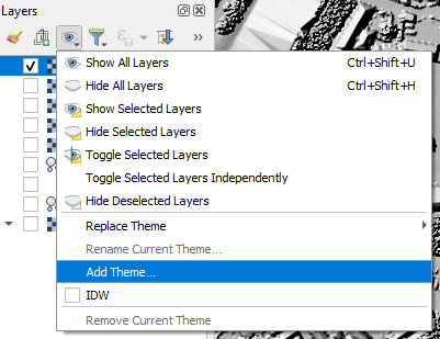
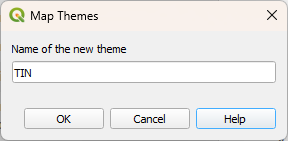
6. In the popup type TIN for the Name of the new theme and click OK.
7. Now click again on the Manage Map Themes and switch between IDW and TIN to compare them.
This also works with a combination of different layers and is useful for demonstrating results. You can also use Map Themes for linking map frames in the Print Layout, for linking 2D and 3D views and for use in field data collection apps, such as Mergin Maps.
In the next section, we'll use the Map Themes to compare two 2D Map Views.
5.2. Compare two 2D Map Views
Now we've set the Map Themes, we can link them to specific 2D Map Views.
1. Close the Layer Styling and Processing Toolbox panels to create more space.
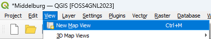
In the main menu, go to View | New Map View.
2. The new map view, with the name Map 1 will dock in a panel. Resize the panel so you have the two map views as big as possible.
3. Use the  icon in the Layers panel to set the Map Theme for the left map (Map 0) to IDW.
4. Use the icon in the toolbar of Map 1 to set the Map Theme to TIN.
The maps are not at the same scale. Let's change that.
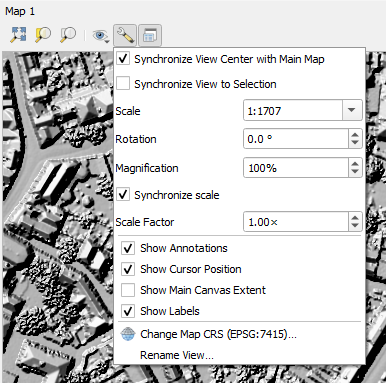
5. In the Map 1 panel click the View Settings  icon and check the boxes to set Synchronize View Center with Main Map and Synchronize scale.
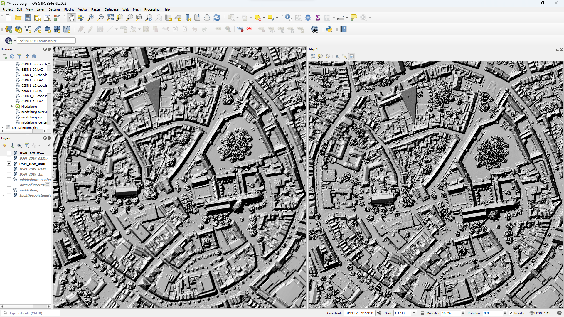
Now the two 2D Map Views are at the same scale and linked:
6. Zoom in at different parts of the map and compare the results.
- Which interpolation gives the best results?
Next, we'll compare the DSM's using the Elevation Profile tool.
5.3. Compare with the Elevation Profile tool
Another way to compare the interpolation results is to use an elevation profile.
1. Close the Map 1 panel.
2. In the main menu go to View | Elevation Profile.
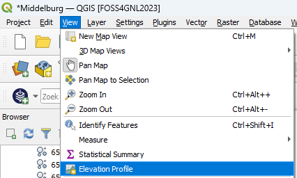
This opens the Elevation Profile panel at the bottom of the map canvas.
3. In the Layer tree, on the left side of the Elevation Profile panel, keep the boxes checked of the layers you want to show in the profile.
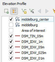
4. Now all the DSM layers have the same colour. Double-click on a line and change the colours so we can distinguish the different lines.

5. Use the Capture Curve  tool to draw a transect line on the map. Click right to end the curve.
6. Compare the different interpolation results.
Note that the VPC layers can't be used. Instead we can add one of the original tiles.
7. Add one or more of the LAZ tiles.
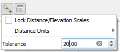
8. Check the elevation profile. Use the Options  icon to change the Tolerance. This determines the buffer around the transect that will include the points in the elevation profile.
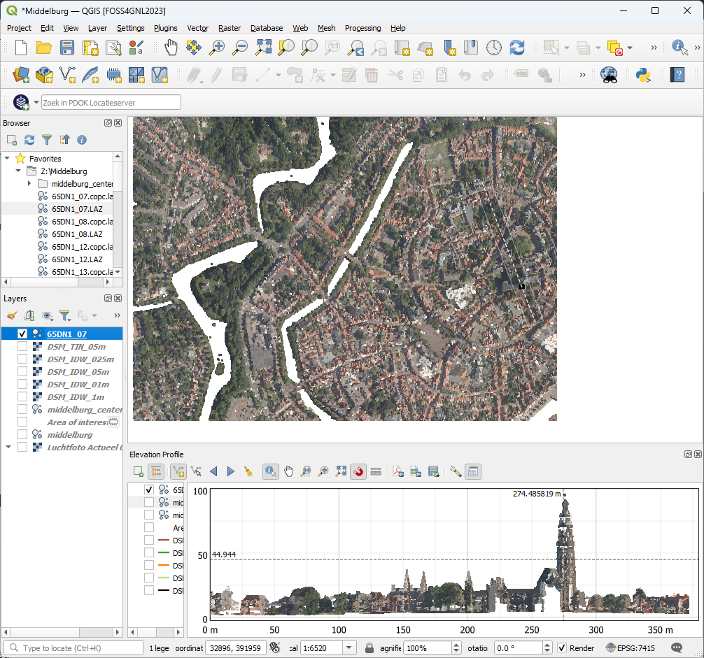
- How high is the church tower (Lange Jan)?
- Compare the points with the interpolation. Which one fits best?