Prepare a basemap
| साइट: | OpenCourseWare for GIS |
| कोर्स: | Planning for Urban Climate Adaptation |
| पुस्तक: | Prepare a basemap |
| द्वारा छापा गया: | अतिथि उपयेागकर्ता |
| दिनांक: | बुधवार, 1 जुलाई 2026, 12:01 PM |
1. Introduction
In this tutorial, we're going to prepare a project in QGIS with some base layers from the internet.
At the end of the tutorial you'll also digitize points, lines and polygons.
After this tutorial, you'll be able to:
- Load vector and raster tiles from the MapTiler plugin.
- Download vector and raster data from OGC services using the PDOK Services plugin
- Download vector data from OpenStreetMap with the QuickOSM plugin
- Download satellite images using the STAC API Browser plugin
- Add 3D vector tiles using the Cesium ion plugin
- Add a land-use map
- Digitize points, lines and polygons
2. Install the MapTiler plugin
1. Start QGIS 3.34 with a new project.
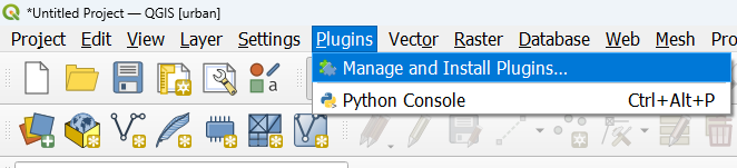
2. In the main menu, go to Plugins | Manage and Install Plugins...
3. Search for MapTiler and install the MapTiler plugin by clicking Install Plugin.

4. Click Close to close the dialog.
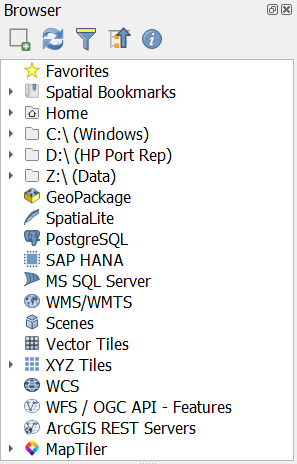
Now you'll see that in the Browser panel a MapTiler folder is added:
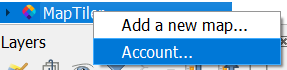
5. Right-click on the folder and choose Account... from the context menu.
6. In the popup dialog, click on the link to create your account and get the token.
7. Copy the token (under Account | Credentials on the MapTiler webpage) and paste it in the dialog in QGIS.

8. Click OK.
9. Setup a new master password for QGIS. This is the password needed to access all passwords and tokens stored in you QGIS profile.
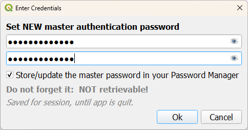
10. Click OK to close the dialog.
In the next section, we'll load a vector tile from MapTiler.
3. Load vector and raster tiles
Let's first load layers that are online available. The easiest way is to load vector and raster tiles from MapTiler.
We'll load a vector tiles layer from OpenStreetMap. Next, we'll add a satellite image as raster tiles.
3.1. Load a vector tile layer
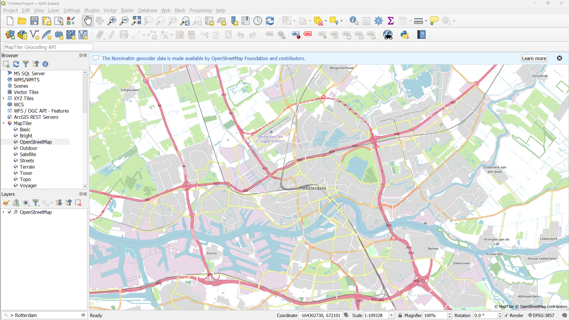
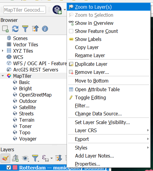
1. Now expand the MapTiler folder in the Browser panel by clicking the little arrow.
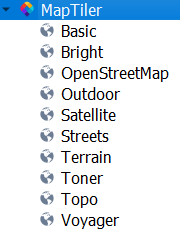
2. Now we can add the the OpenStreetMap vector tile layers by clicking right and selecting Add as Vector from the context menu.

When there's an warning at the top of your screen, click the cross to remove the message.
Now we need to find Rotterdam. We'll use the built-in geocoder of QGIS, which uses the Nominatim database from OpenStreetMap.
3. In the Locator bar type
> Rotterdam
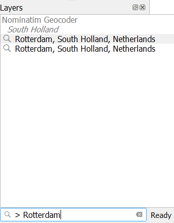
4. Double-click one of the options and you'll automatically zoom to the area.
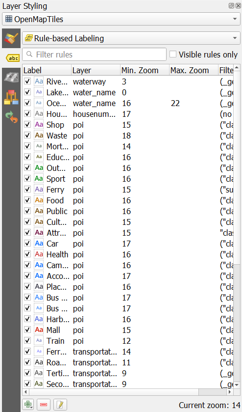
3.2. Modify the style of a vector tile
1. In the Layers panel, expand the OpenStreetMap group by clicking the little arrow.

2. Click on the OpenMapTiles layer to select it.
3. Click the  icon to open the Layer Styling panel.
The map has too much detail. We'll hide elements that we don't want to see.
4. At the Symbology tab, experiment with unchecking points, lines and polygons to see what's in the city and what you want to visualise.

5. If you click on a symbol, you can change it's properties, for example colour or line thickness.
Note that visibility is also controlled by the zoom level, which you can edit here.
You can also control the labels.
6. Go to the Labels tab and uncheck labels that you want to hide. If you click on a label you can change its properties.
- Can you modify the map in such a way that you highlight blue and green infrastructure in the city?
Feel free to explore the other MapTiler vector tiles. There are even more available if you right-click on MapTiler and choose Add a new map... from the context menu.
You could try the NL ones here:

3.3. Load a satellite image
Besides vector data, we can also load raster data.
Let's add a high resolution satellite image.
1. In the Browser panel go to the MapTiler folder and click right on Satellite.
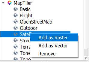
2. Choose Add as Raster from the context menu to add the Satellite image raster tile to the map canvas.
3. In the Layers panel, uncheck the box of the OpenStreetMap group to hide the OpenMapTiles vector tile and see the satellite image below.
4. Zoom in to see the details.
- Can you see the blue and green infrastructure?
- How does this relate to the vectors you have previously visualized?
4. Download vector and raster layers
Until now, we've only viewed online layers. This is nice for quick visualizations. For analysis, however, we need local data.
For the Netherlands a lot of data is freely available through the PDOK Services plugin. In the next sections, we'll install the plugin and download the following layers:
- Municipality boundary
- Digital Surface Model
- Digital Terrain Model
In addition, we'll download building footprints from OpenStreetMap.
4.1. Install the PDOK Services plugin
Let's first install the PDOK Services plugin that gives us access to a lot of open data from the Dutch government. Data are available as WMS, WMTS, WFS, WCS and OGC:API tiles and features.
1. In the main menu, go to Plugins | Manage and Install Plugins....
2. Search for the PDOK Services plugin and click Install Plugin.
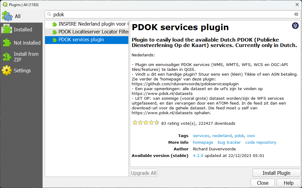
3. After installing click Close to close the dialog.
Now you'll see that the PDOK Services toolbar has been added to QGIS.

In the next sections, we'll use it to download vector and raster layers.
4.2. Download the municipality boundary
For our study of Rotterdam, we need the boundary polygon of the municipality. For that purpose, we first need to download a vector layer with all municipalities of the Netherlands, select Rotterdam and export it to a new vector layer for our database. We need a WFS (Web Feature Service) to get the vector data.
1. In the toolbar, click on  to open the PDOK Services Plugin dialog.
2. There, search for Gemeenten, WFS, the newest version. Use the Zoeken field, which means search in Dutch.

3. Click Boven to add the layer to the top of the Layers panel.
4. Click Close and wait until the layer loads.
Now we need to select the municipality of Rotterdam.
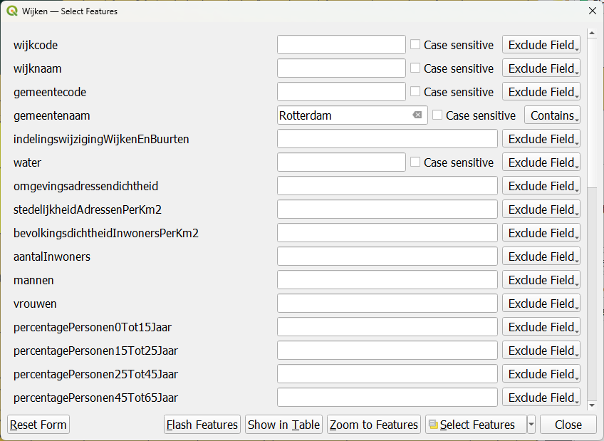
5. In the toolbar click Select Features by Value....

6. In the Select Features dialog type Rotterdam at gemeentenaam (municipality name). If you start typing it will automatically complete and you can select the name.
7. At water type NEE. This is to select only the land part of the municipality and not extend it into the sea.

You can see that this layer has a lot of attributes. It is census data. We'll look at that later.
8. Click Select Features to select this polygon.
9. Click Close to close the dialog.
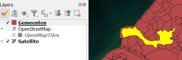
Now you'll see that one polygon is highlighted in yellow. That's the municipality boundary polygon of Rotterdam.
Now we need to export the selection to a database where we want to store our data for Rotterdam.
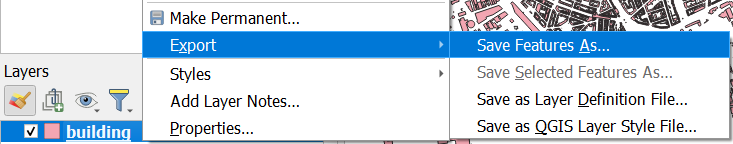
10. In the Layers panel, right-click on the Gemeenten layer and choose Export | Save Selected Features As....

11. In the Save Vector Layer as dialog, make sure to choose the GeoPackage format. Then use the Browse  button to browse to the folder where you want to store your GeoPackage. Save it as Rotterdam.gpkg. Change the Layer name to municipality boundary.

12. Leave the rest as default and click OK.
13. In the Select Transformation dialog click OK to accept the default.

This appears, because the projection of the project is different from the layer. The project projection is Pseudo Mercator (EPSG:3857), which is the projection of the online layers we've loaded before. The municipality layer is in the Dutch projection, EPSG: 28992 and has to be on-the-fly reprojected to Pseudo Mercator.
To work in the correct projection, also visually in the map canvas, we'll now change the on-the-fly reprojection to the Dutch projection.
14. In the lower right of the window, click on the EPSG code.

15. In the Project Properties - CRS dialog type 28992 at Filter. This is the EPSG code of the Dutch projection.
16. Select Amersfoort / RD New under Predefined Coordinate Reference Systems.
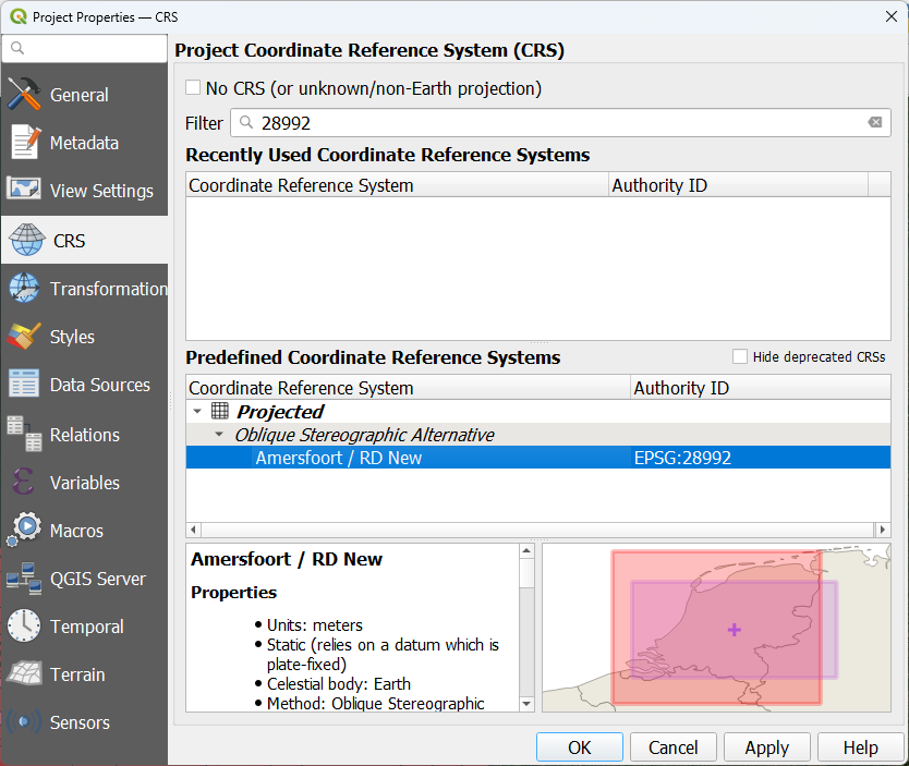
17. Click OK to apply and close the dialog.
Now the map canvas in the Dutch projection.
Let's clean up a bit before we continue.
18. In the Layers panel, right-click on the Gemeenten layer and choose Remove layer... from the context menu. In the popup, click OK to confirm.
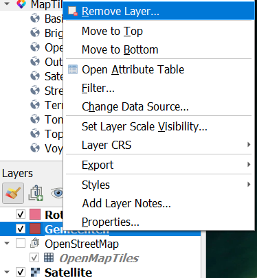
Now the layer with all municipalities of the Netherlands is removed.
19. In the Layers panel, right-click on the Rotterdam - municipality boundary layer and choose Zoom to Layer(s).
Let's now style the boundary with a line.
20. Go to the Layer Styling panel. Make sure that the Rotterdam - municipality boundary layer is the active layer.
21. Select Simple Fill.
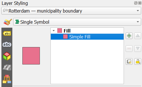
22. Change it the Symbol Layer Type to Outline: Simple line. Change the color to red and give it a thickness of 0.66 mm.

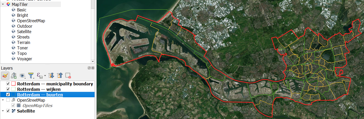
23. Repeat this for the WFS layer Wijken (quarters) and Buurten (neighbourhoods).
After loading the WFS you select the features based on Gemeentenaam Rotterdam and export them to the database with layer names quarter and neighbourhoods. Style them with different line colours and thickness.
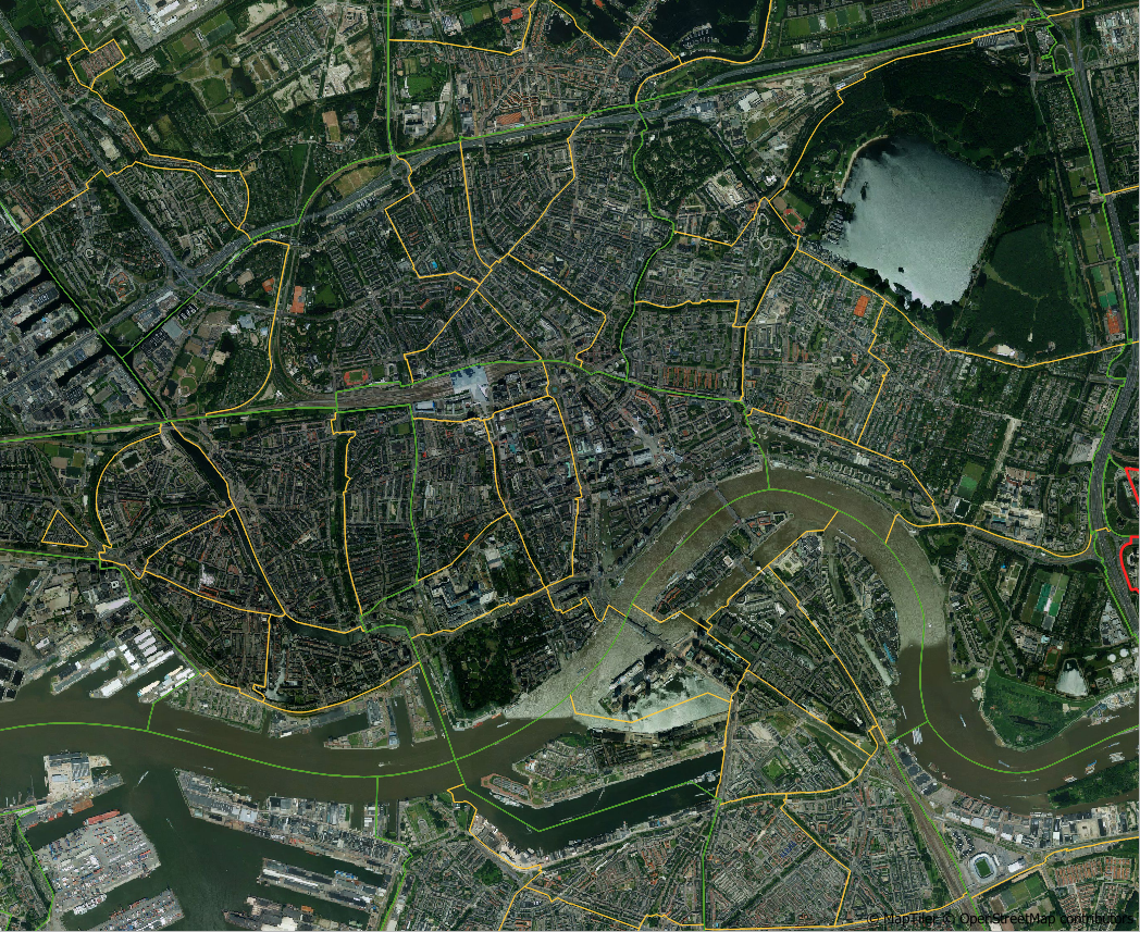
In the end your map canvas should look like this:
Now is a good moment to save your project. Regularly save your project to avoid data losses.
23. In the main menu, go to Project | Save To | GeoPackage....
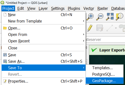
24. In the Save project to GeoPackage popup dialog, use the  button to locate your GeoPackage (Rotterdam.gpkg) and save the project as Rotterdam.
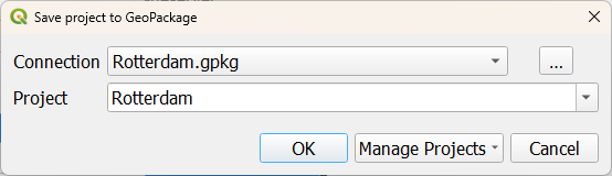
25. Click OK.
Next, we'll add the Digital Surface Model and Digital Terrain Models.
4.3. Download elevation rasters
Now we're going to download two raster layers: a Digital Surface Model and a Digital Terrain Model. We'll again use the PDOK Services plugin.
1. In the toolbar, click  to open the PDOK Services dialog.
2. Search for AHN (Actueel Hoogtebestand Nederland, which is the Dutch elevation model).
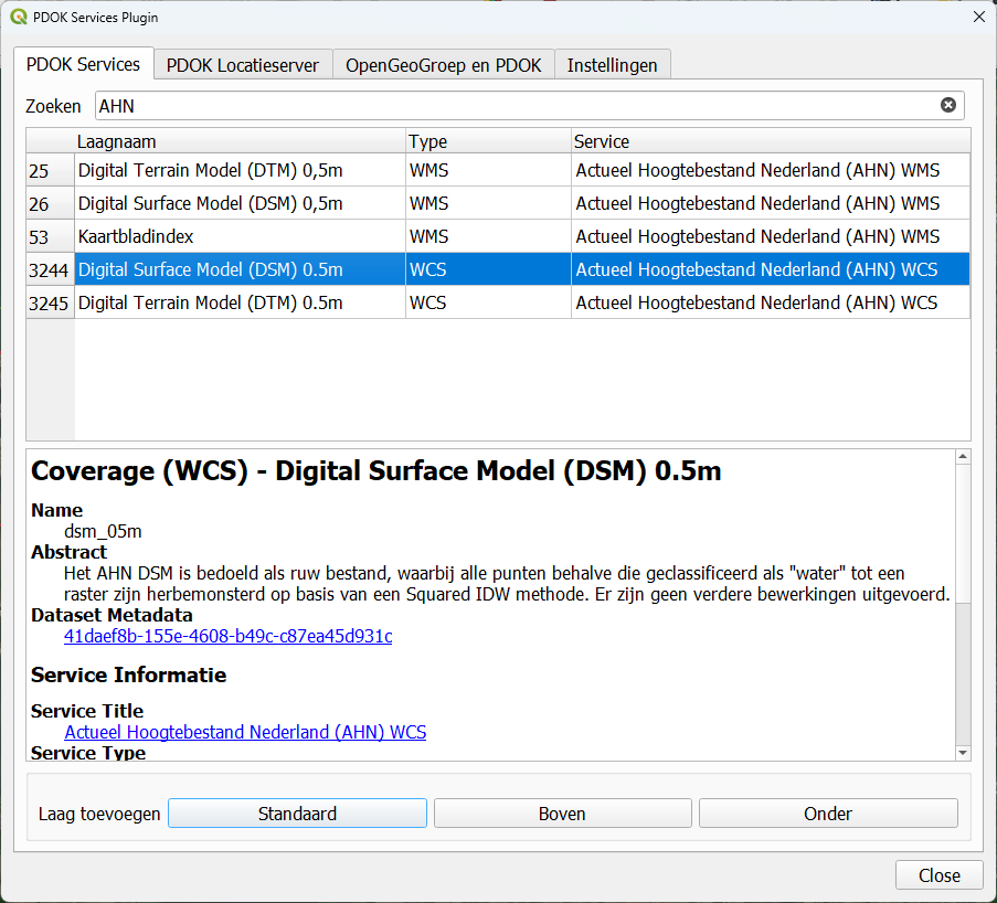
3. There select the Digital Surface Model 0,5m in WCS format and click Boven to add it to the top of the Layers panel.
4. Click Close to close the dialog and wait until the layer is loaded.
Let's clip the downloaded layer to a smaller area. The pixels of this raster are 50 cm, so you'll need a lot of disk space to download the whole municipality. We're mostly interested in the center of Rotterdam.
5. Zoom in to a smaller area around the center of Rotterdam.
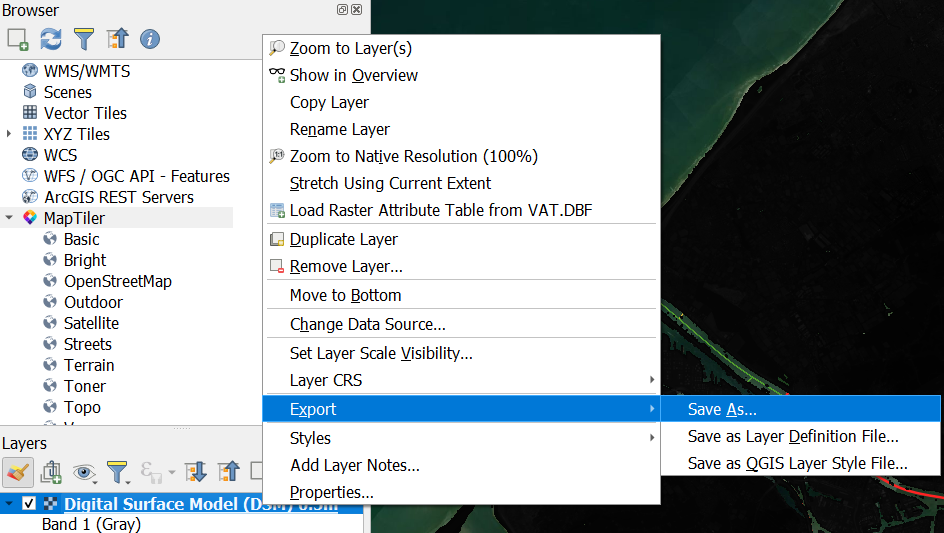
6. Right-click on the Digital Surface Model layer and choose Export | Save as... from the context menu.
6. In the Save Raster Layer as... dialog Save the result to DSM_Rotterdam.tif in the same folder as your GeoPackage. Under Extent click Map Canvas Extent.
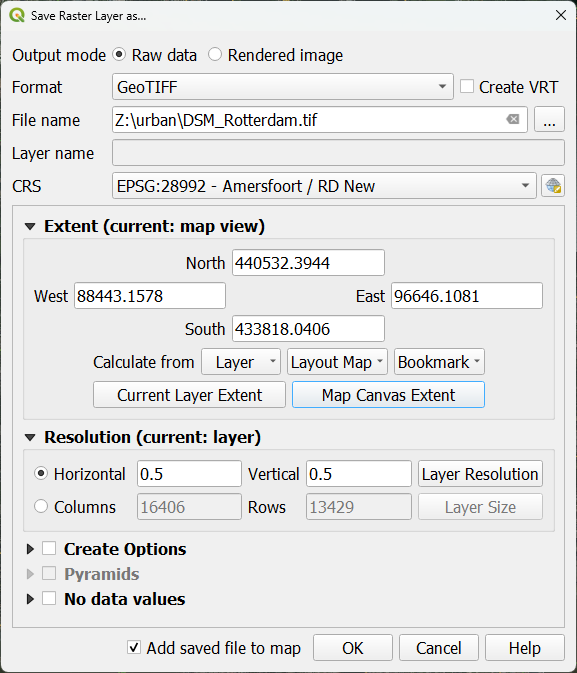
7. Keep the rest as default and click OK.
8. When it's done, remove the Digtial Surface Model WCS layer.
Let's style the result.
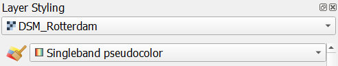
9. Go to the Layer Styling panel and make sure that DSM_Rotterdam is the active layer.
10. Change the renderer from Singleband gray to Singleband Pseudocolor.
11. At Color ramp choose Turbo.
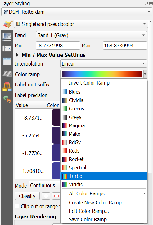
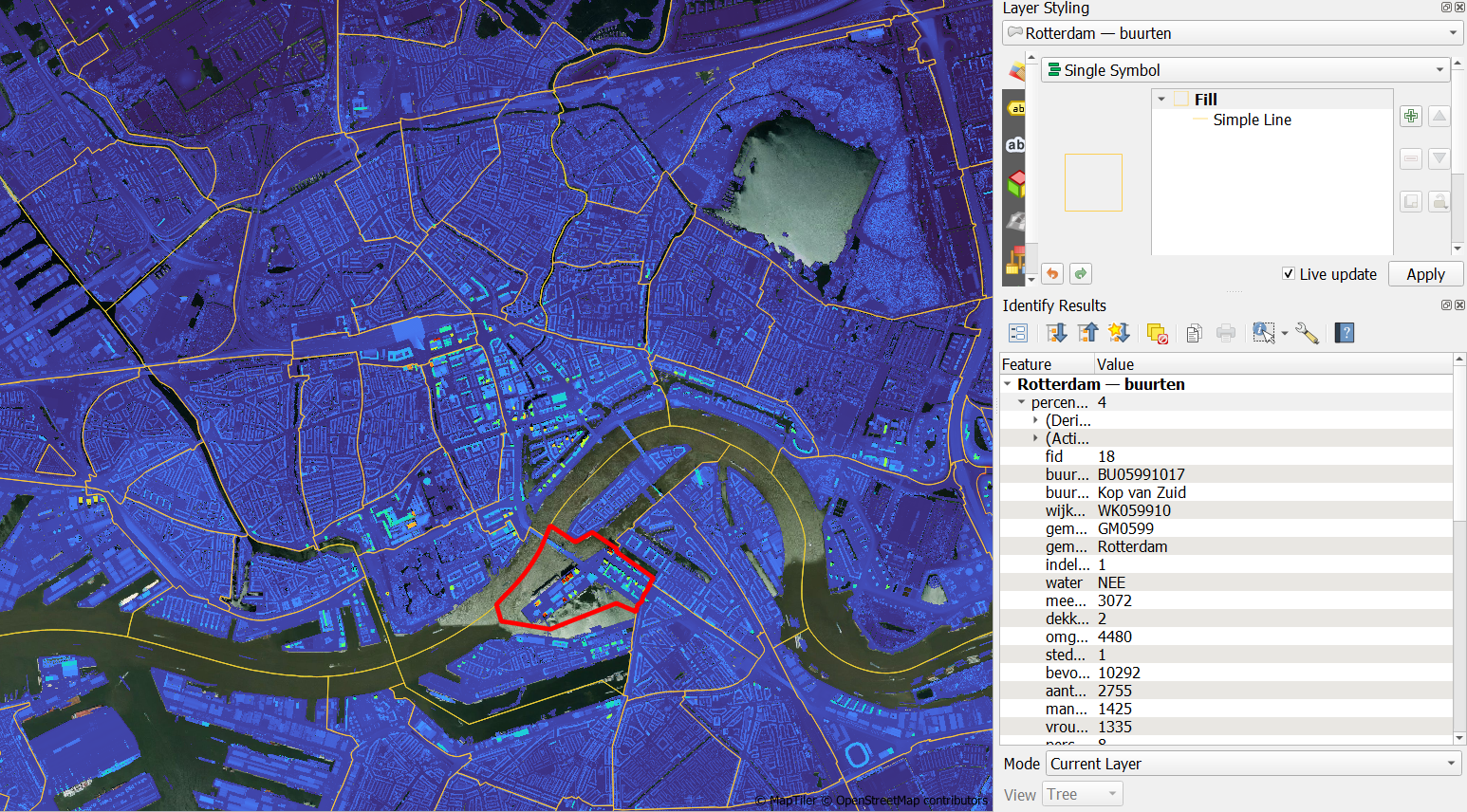
12. Inspect the result.
- Which neighbourhoods have the tallest buildings?
- Where do we find neighbourhoods with low elevations?
Tip: overlay the neighbourhood layer and use the Identify tool  to find the name of the neighbourhood.
13. Repeat this for the Digital Terrain Model and save it as DTM_Rotterdam.tif.

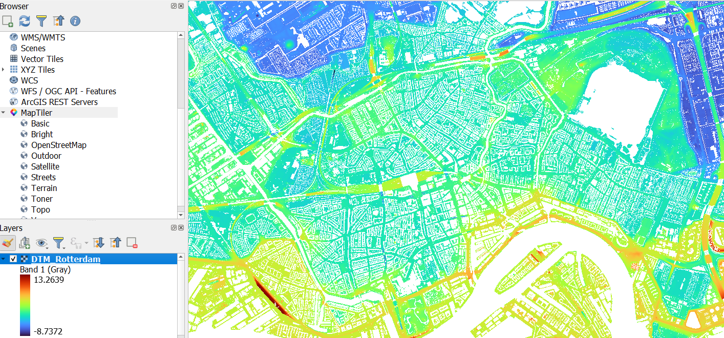
- Which pixels have nodata?
4.4. Download buildings
In this section, we'll download buildings. In this case we'll use OpenStreetMap. We can download buildings from OpenStreetMap with the QuickOSM plugin.
This video shows how the plugin works:
1. Install the QuickOSM plugin.
2. In the toolbar, click  . Accept the license agreement in the popup.
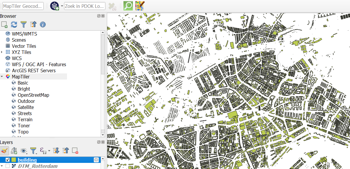
3. In the QuickOSM dialog, type at Key building. Leave Value blank, so it will download all buildings. Click In and choose Canvas Extent. Then under Advanced uncheck the boxes for Points, Lines and Multilinestrings so we only download Polygons. Then click Run query. If the area is too large, zoom in a bit bore in the map canvas.

Now you see all buildings in the map canvas.
Note the  icon next to the layer. This means that the layer is a temporary scratch layer and that it can be lost if QGIS is closed. We have to make it permanent if we want to keep it.
One way is to click on the  icon. With this method, however, we can't control the output projection. It is good practice to reproject the layer immediately to the projection that we need.
5. Right-click on the building layer and choose Export | Save Features As... from the context menu.
6. In the dialog, save the layer as buildings in the Rotterdam.gpkg GeoPackage. Change the CRS to the one of the project (EPSG:28992).
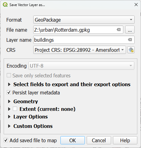
7. Click OK.
Now your buildings are stored in the GeoPacakge.
8. Remove the temporary building layer.
9. Save the project by clicking  .
.
- Now use the QuickOSM plugin to download other relevant points, lines and polygons for climate adaptation research of Rotterdam. Use key/values that you can find on this page: Map features - OpenStreetMap Wiki. Style them and store them in your GeoPackage.
5. Load a false colour image
In this chapter we'll add a false colour aerial photograph to our project. In the image, the near infrared band is visualized in red, which makes it easy to find areas with healthy vegetation. The image is available from the PDOK Services plugin.
1. Click  to open the PDOK Services plugin dialog.
2. Search for Luchtfoto Actueel Ortho 25cm Infrarood. This is a WMTS layer, which means it is a WMS layer in tiles, which is useful for visualization only.
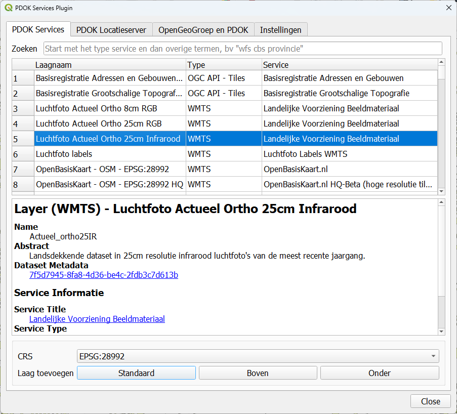
3. Click Boven to add the layer to the top of the Layers panel.
- Explore the false colour aerial photograph. Check where the green infrastructure of the city is located.

6. Download satellite data
With satellite data we can explore other parts of the electromagnetic spectrum that are not visible to human eyes. We're going to download:
- A multispectral image (Sentinel 2)
- A temperature product
6.1. Download a multispectral satellite image
With satellite data we can explore other parts of the electromagnetic spectrum that are not visible to human eyes. We're going to download a Sentinel image using the STAC API Browser plugin.
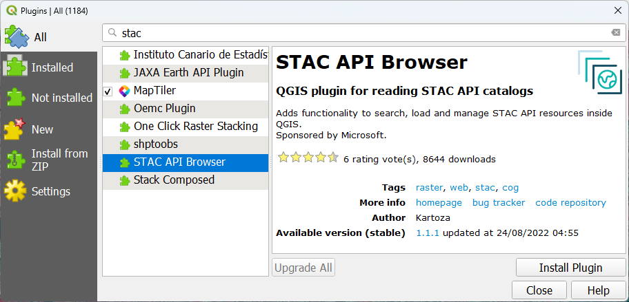
1. Install the STAC API Browser plugin.
2. Zoom to the boundary of the municipality.
3. Click  to open the STAC API Browser dialog.
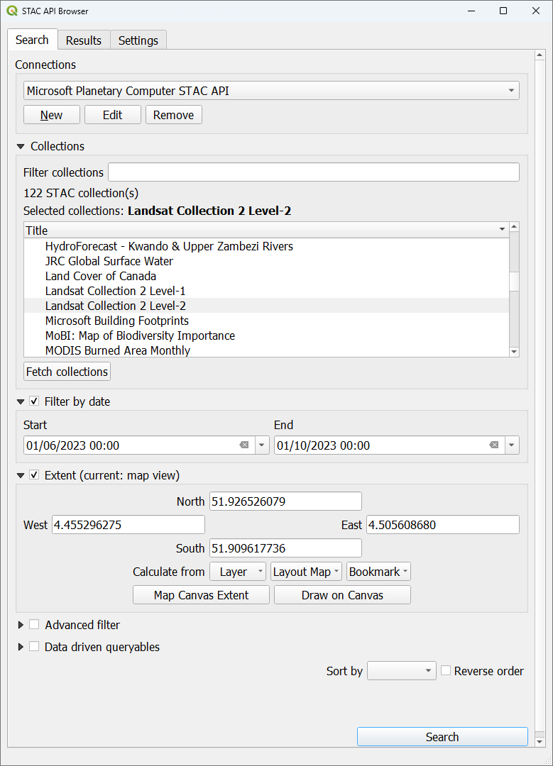
4. At Connections, choose Microsoft Planetary Computer STAC API.
5. Click Fetch Collections.
6. Select Sentinel-2 Level-2A.
7. Check the box to Filter by date and give a date range from 1 June 2023 - 1 October 2023.
8. Check the box for Extent and click Map Canvas Extent.

9. Click Search.
10. Check the results. We're looking for an image without cloud cover over Rotterdam.
The image of 6 September 2023 looks good.
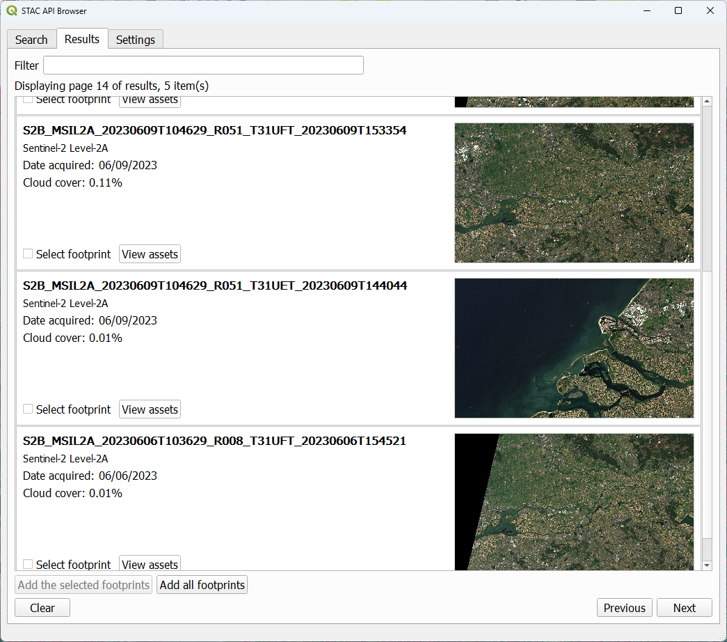
11. At the image of 6 September 2023 click View assets.
12. In the Assets dialog check the boxes to Select to add as layer for bands 2, 3, 4 and 8, which are the visual and near infrared bands.
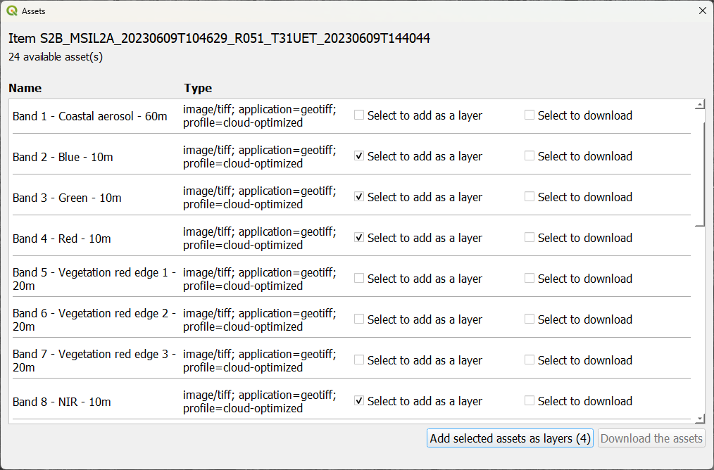
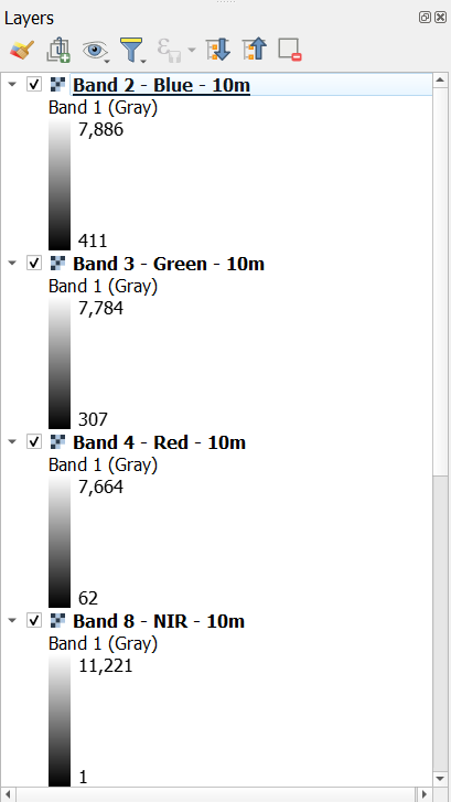
13. Click Add selected assets as layers (4) to add them to the map canvas.
14. Order the layers in the Layers panel so that band 2 is on top and band 8 is at the bottom.
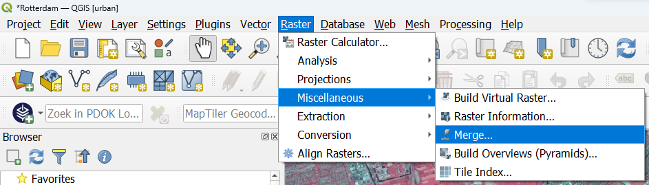
We need to stack these bands in order to visualize them with the Multiband color renderer.
15. In the main menu, go to Raster | Miscellaneous | Merge....
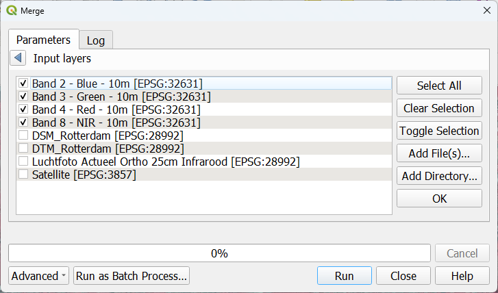
16. In the Merge dialog, click  to select the input layers. Select bands 2, 3, 4 and 8 and click
  to go back.
17. Back in the Merge dialog, check the box to Place each input file into a separate band. This will create the stack (multiband) raster.
18. Save the result as Sentinel2_060923.tif and click Run.
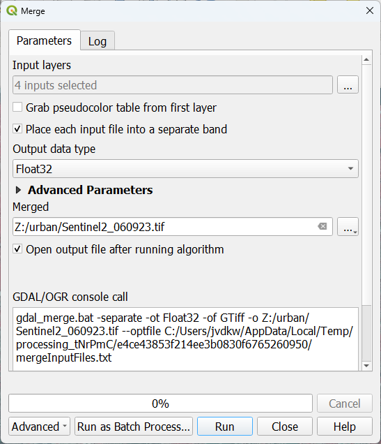
19. Click Close after processing.
20. Remove the layers with the individual bands.
21. Go to the Layer Styling panel. Make sure that the Sentinel2_060923 layer is the active layer.
22. Use the Multiband color renderer to visualize different band combinations.
23. To create a false colour image, similar to the aerial photograph, choose for
- Red: Band 4 (this is the Near Infrared band)
- Green: Band 3 (this is the Green band)
- Blue: Band 2 (this is the Blue band)
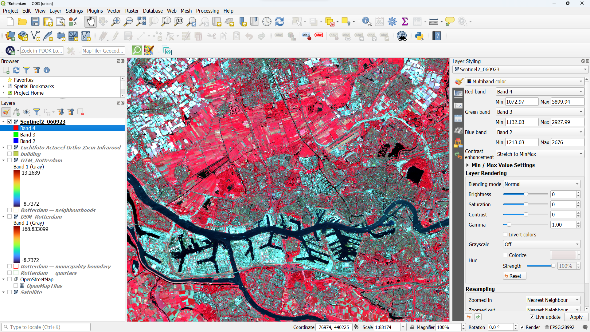
- Check the result. Zoom in to different areas of the city.
- Compare the satellite false colour image with the aerial photograph. What do you observe?
This video shows how the STAC API Browser can be installed and used:
6.2. Download a temperature image
In this section, you'll learn to add a temperature image to your project.
1. Go back the STACK API Browser plugin dialog.
2. Choose Microsoft Planetary Computer STAC API at Connections.
3. Click Fetch collections.
4. Select Landsat Collection 2 Level 2.
5. Filter by date from 1 June - 1 October 2023.
6. Choose the Map Canvas Extent (make sure you're still zoomed to Rotterdam)
7. Click Search.
8. Look for the image of 9 September 2023 and click View assets.

9. Go to the line of the Surface Temperature band and check the box to Select to add as layer.

10. Click Add selected assets as layers (1).
11. Close the dialogs and check the result in the map canvas.
- What are the units of the Surface Temperature product?
- What is the spatial resolution of the Surface Temperature product?
The values need to be scaled to get the temperatures in Kelvin. You can find more information at this page. It is always important to check the documentation of data sets! Furthermore we want to have the temperatures in degrees Celcius.
12. In the main menu, go to Raster | Raster Calculator....
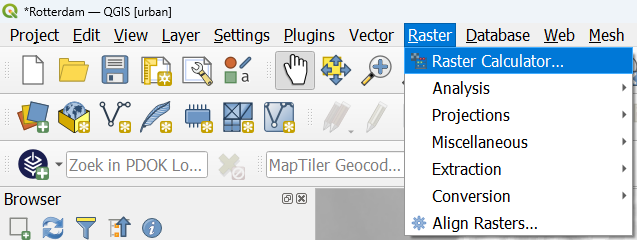
13. In the Raster Calculator, double click under Raster Bands on Surface Temperature Band@1 to add it to the Raster Calculator Expression.
14. Compose the following expression:
( "Surface Temperature Band@1" * 0.00341802 + 149.0 ) - 273.15

15. Save the result in your project folder to T_Celsius_09092023.tif. In this way we can easily recognize that it is temperature in Celsius and the date of the image.
16. Click OK.
17. Remove the original Surface Temperature Band layer.
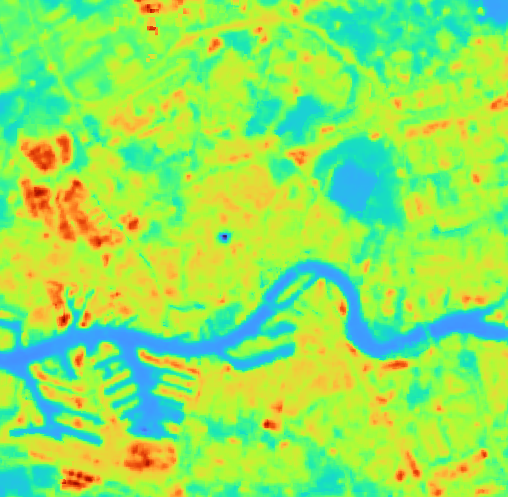
18. Select the new T_Celsius_09092023 layer and open the Layer Styling panel.
19. Change the renderer to Singleband Pseudocolor and choose the Turbo color ramp. In that way, blue is for cold pixels and red is for warm pixels.
The contrast in the image can be improved.
20. Expand the Min / Max Value Settings by clicking the black arrow.
21. There click the radio button before Min / Max and change the Statistics Extent from Whole raster to Current canvas.
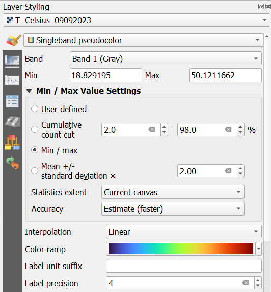
Now the minimum and maximum values of the extent of the map canvas will be used, increasing the contrast. Note that with Updated canvas, the min/max values will be updated when you pan, which will keep the maximum contrast.
- Where are the cold and hot spots in the city?
7. Add 3D vector tiles
Since QGIS 3.34 there is support for 3D Tiles. In this chapter we're going to load the Google Photorealistic 3D Tiles into QGIS. They are available through the Cesium ion plugin.
To limit memory usage, we're first going to limit the extent of our project to the main area of interest.
1. Make sure you're zoomed in to the main area of interest.
2. In the main menu, go to Project | Properties....

3. In the Project Properties dialog go to the View Settings tab and check the box before Set Project Full Extent.
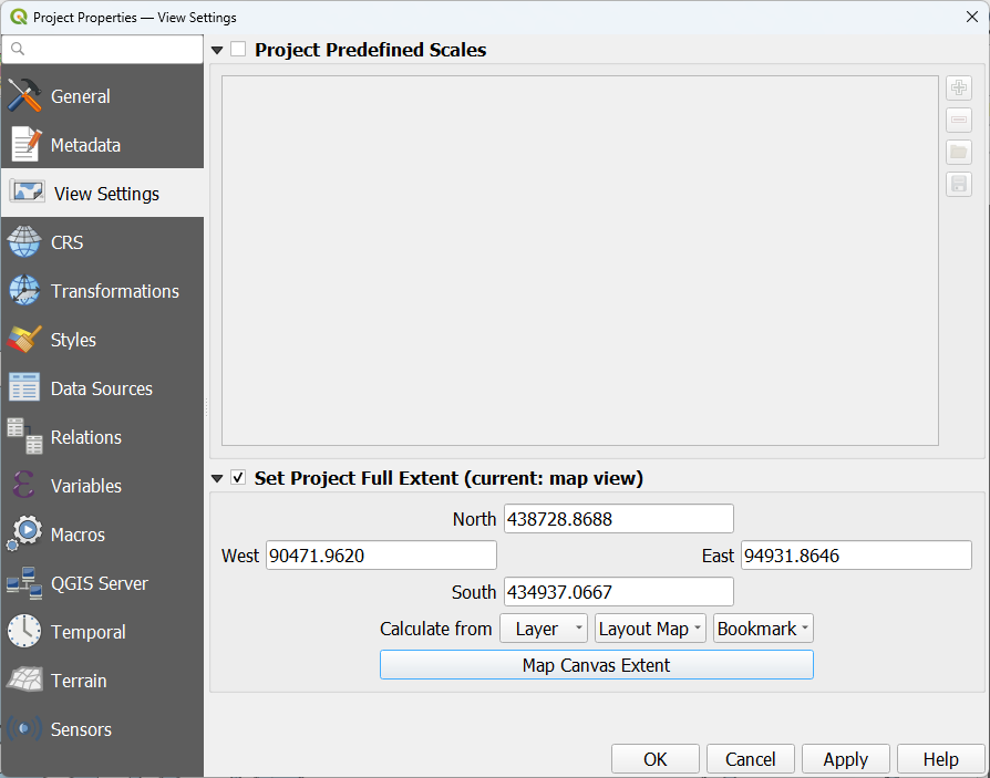
4. Click Map Canvas Extent to set the limits to the current map canvas.
Now we can install the Cesium ion plugin and search for 3D tiles.
5. Install the Cesium ion plugin.
6. In the Browser panel, click on the Cesium ion folder. Your internet browser will open and ask you to login. Use one of the options to login and accept the necessary permissions that QGIS needs.
7. Go back to the Browser panel and add Google Photorealistic 3D Tiles to the map canvas.
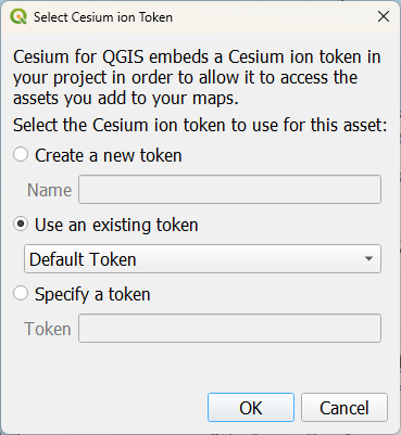
8. A popup will show up to ask which token you want to use. Keep the default to Use an existing token and click OK.
Now the 3D tiles are loaded in the 2D view.
Although they are nice in 2D they are more impressive in 3D.
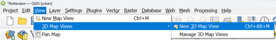
9. In the main menu, go to View | 3D Map Views | New 3D Map View.
10. In the 3D Map View, click the scroll button of your mouse and drag it towards you to tilt the scene. Now us the left mouse button to pan and navigate through the study area.
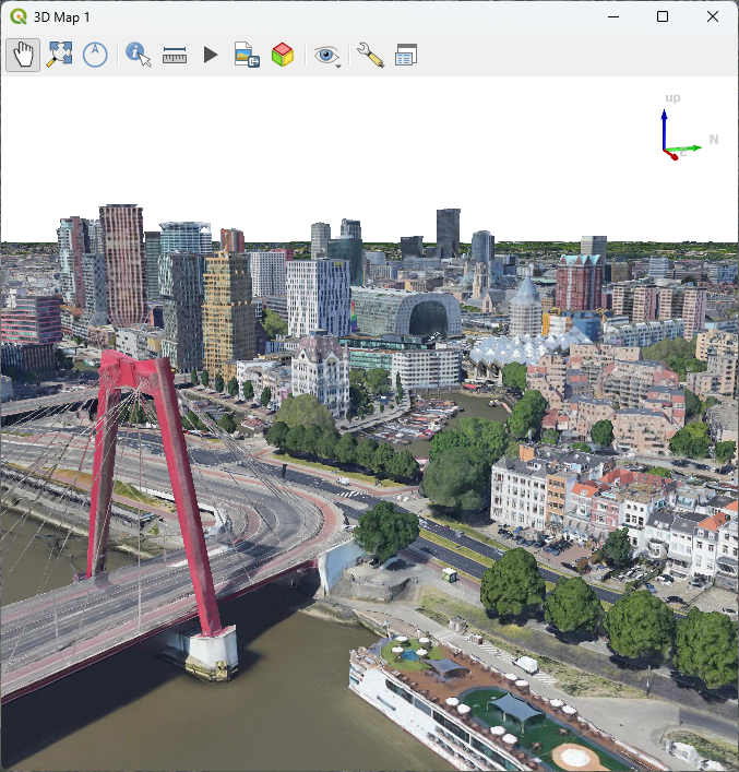
This video shows the procedure:
8. Add a land-use map
Here we'll add the land-use map of the Netherlands: LGN 2022 (https://doi.org/10.4121/688363cc-8c79-439f-bb0e-fe5d0deb3161). For global datasets, see here.
LGN data can be downloaded here, but you can best download it from the main course page, because for QGIS 3.34 the style files do not work (bug) and another file is provided. The provided file is also clipped to the boundary of the municipality of Rotterdam, to reduce its file size.
1. Download the data from the main course page. Make sure that you unzip the folder in your project folder before use.
2. Locate the LGN2022_Rotterdam.tif file in the Browser panel and drag the layer to the map canvas.
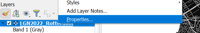
3. In the Layers panel, right-click on the LGN2022_Rotterdam layer and choose Properties... from the context menu.
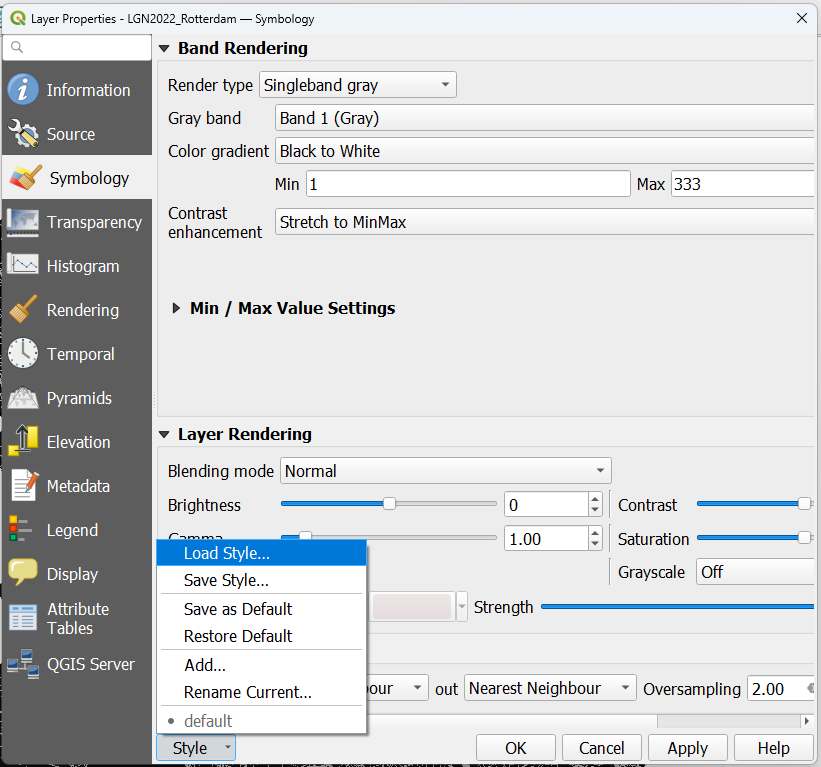
4. In the Layer Properties dialog go to the Symbology tab.
5. At the bottom of the dialog, choose Style | Load Style....
6. Use the browse  button to locate legend.qml, which is provided.
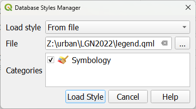
QML files are QGIS files that contain styling.
7. Click Load Style.
The classes are loaded. The names were originally in Dutch, but have been translated.
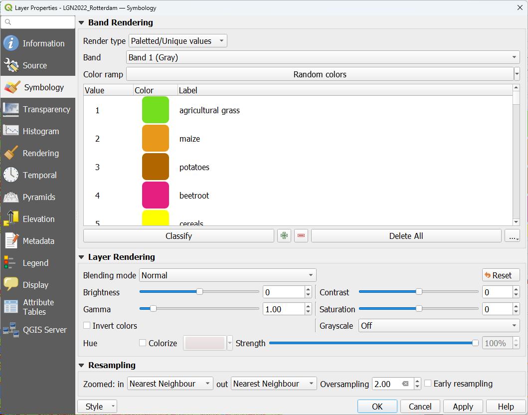
8. Click OK to close the dialog.
Have a look at the land use in Rotterdam.
9. Digitize features
Besides having base layers from external sources, you can also add your own points, lines and polygons by digitization.
Watch these videos on digitizing and styling points, lines and polygons in QGIS:
- Digitize points, lines and polygons of features related to nature based solutions and climate adaptation.
10. Conclusion
In this tutorial, we've built the database for our studies on urban water challenges.
In the next tutorials, you'll use these datasets. Make sure to save your project.