Tutorial: GIS for adaptation
| Site: | OpenCourseWare for GIS |
| Course: | Planning for Urban Climate Adaptation |
| Book: | Tutorial: GIS for adaptation |
| Printed by: | Guest user |
| Date: | Monday, 13 July 2026, 2:24 AM |
1. Introduction
In this tutorial, we're going to calculate a few urban metrics.
We'll use the neighbourhoods, quarters and buildings layers of the previous tutorial as well as the land-use raster.
1. Open the project of the previous tutorial.
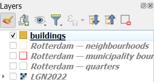
2. Remove all layers, except the buildings, neighbourhoods, municipality boundary, quarters and LGN2022.
3. Save your project to the GeoPackage under a new name, for example Metrics.
2. Calculate areas and densities
In this chapter we're going to calculate areas and densities.
This requires the following steps that will be elaborated in the next sections:
A. Calculate the areas of the neighbourhood polygons
B. Add the neighbourhood names and areas to the buildings
C. Dissolve the buildings that are from the same neighbourhoods
D. Calculate the areas of the dissolved building polygons
E. Divide the area of dissolved building polygons by the area of the neighbourhoods
2.1. Calculate areas of neighbourhoods
In this section, we're going to calculate areas of neighbourhoods.
1. In the Layers panel, right-click on the neighbourhoods layer and choose Open Attribute Table from the context menu.

2. In the attribute table, click  to toggle on the editing mode.
3. Click  to open the Field Calculator.
4. Create a new field with the Output field name Area (m2) and Output field type Decimal number (real).
5. Under expression add $area.
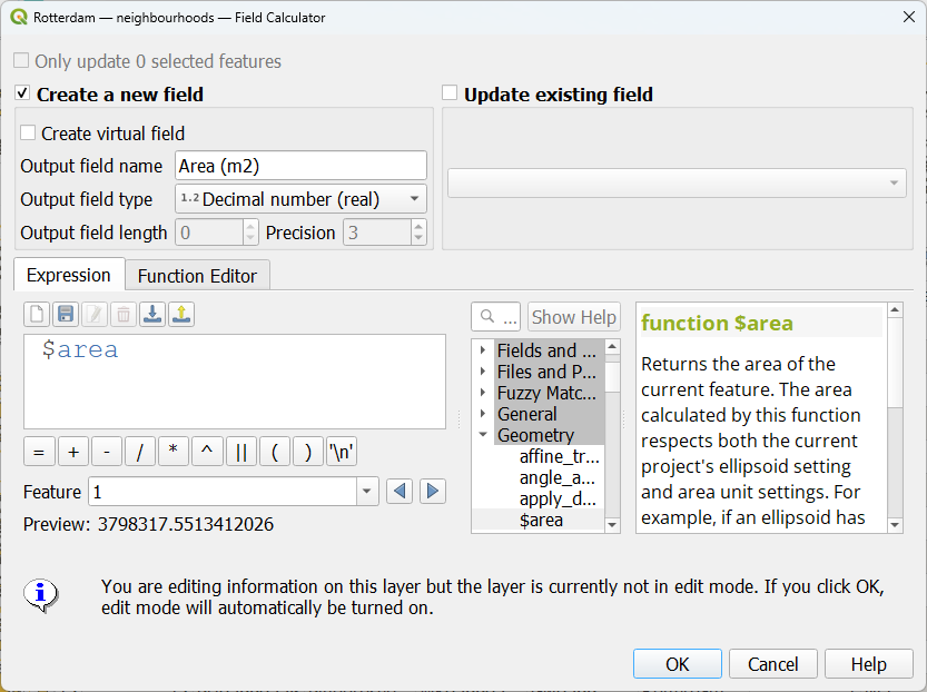
6. Click OK.
Now you'll see that the area of the neighbourhood polygons is added to the attribute table.
7. Click to toggle off editing. Confirm that you want to save the results.
In the next section, we're going to add this information to the building polygons.
2.2. Spatial join
In order to add the the neighbourhood names and areas to the building attributes we need to join the attribute tables.
In this case, there's no common key field that we can use, so we have to do a so-called spatial join. We assume that all buildings are within one neighbourhoud.
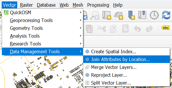
1. In the main menu, go to Vector | Data Management Tools | Join Attributes by Location....
2. Choose to Join to features in buildings that intersect with neighbourhoods.
3. Choose buurtnaam (name of the neighbourhood) and Area (m2) as fields to add.
4. For Join type, keep Create separate feature for each matching feature (one-to-many).
5. Save the result in the GeoPackage as buildings with neighbourhoods.
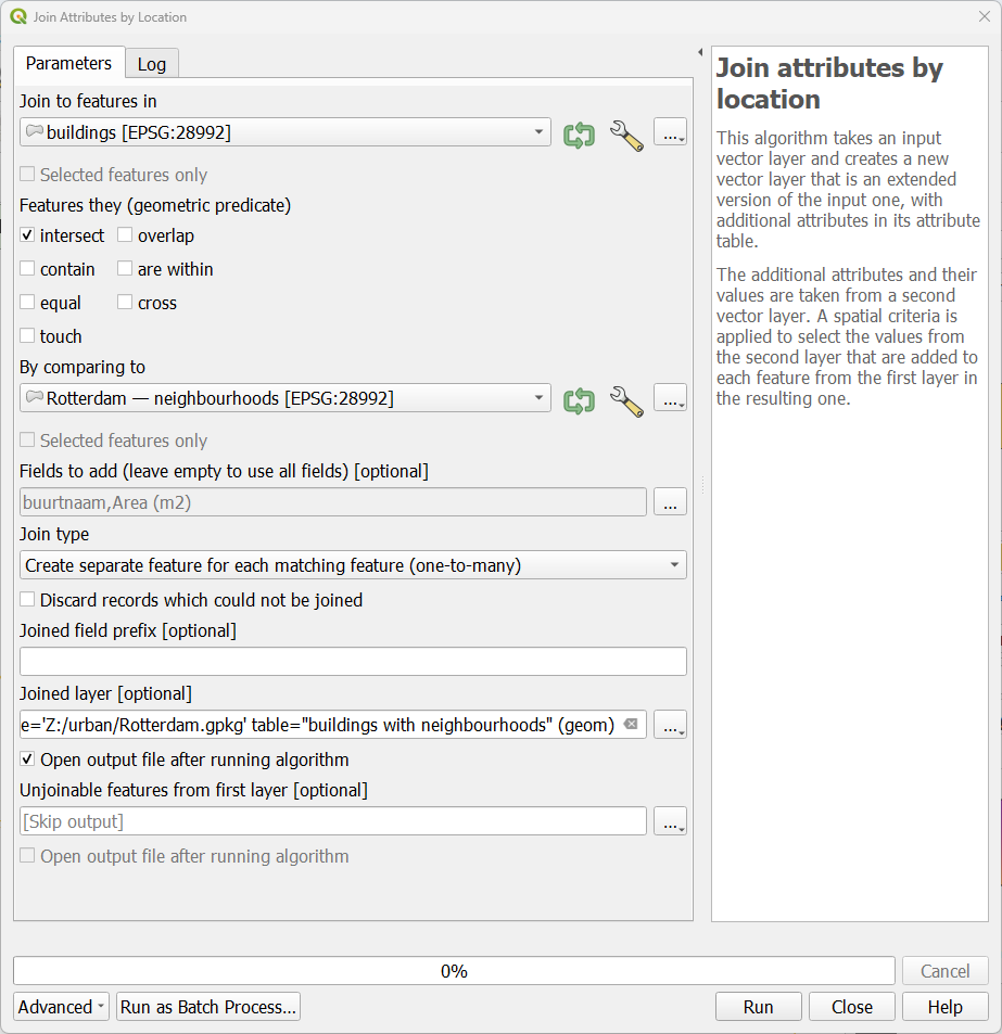
6. Click Run. Click Close when the processing is completed.
7. Check the attribute table of the buildings with neighbourhoods layer.
Next, we're going to dissolve all buildings that belong to the same neighbourhood.
2.3. Dissolve features
Now each building has the name and surface area of the neighbourhood to which it belongs.
In order to calculate the building density, we need to calculate the total surface area of the building in each neighbourhood. Therefore, we first need to dissolve the building polygons, based on their neighbourhood name attribute.
1. In the main menu, choose Vector | Geoprocessing Tools | Dissolve....

2. In the Dissolve dialog, choose buildings with neighbourhoods as Input layer, choose buurtnaam as the Dissolve field and save the result to the GeoPackage with the name buildings dissolved.
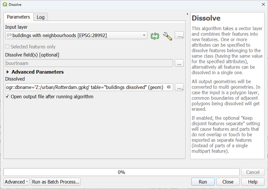
3. Click Run. Click Close after processing has completed.
Let's check the result visually.
4. In the Layers panel, select the buildings dissolved layer.
5. Go to the Layer Styling panel.
6. Change the Single Symbol renderer to Categorized. Choose buurtnaam for Value.
7. Click Classify.
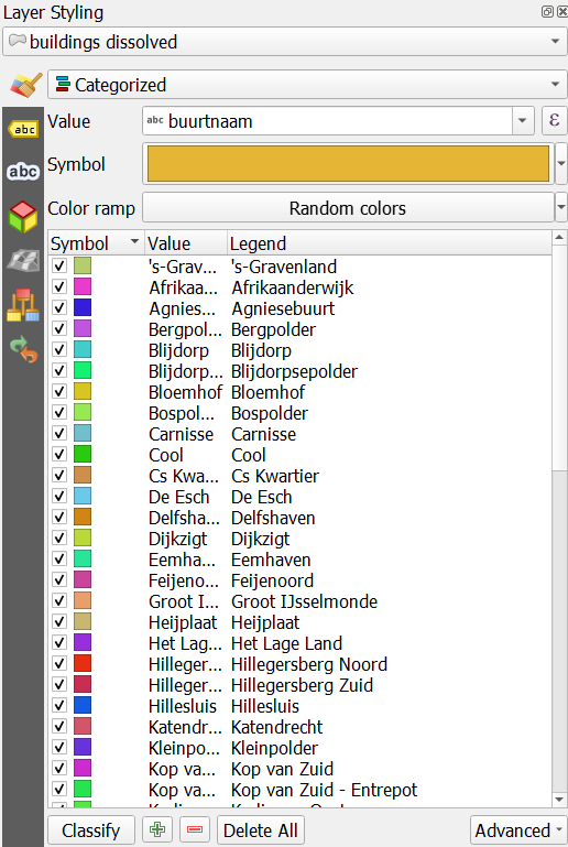
Now all buildings of the same neighbourhood have the same random colour.

2.4. Calculate densities
To calculate the building density per neighbourhood, we need to first calculate the total area of the buildings per neighbourhood.
In Section 2.1 of this tutorial, you have already calculated the area of neighbourhoods.
1. In the same way, use the Field Calculator to calculate the area of the dissolved building features. Call the new field Building area (m2).

Now we can calculate the percentage of buildings per neighbourhood.
2. Go to the Field Calculator of the buildings dissolved attribute table.
3. Create a new field with the name building percentage with the Output field type Decimal number (real).
4. Create the following expression: (use the middle panel of the dialog, under Fields and Values double click on the fields you want to add to the expression)
"Building area (m2)" / "Area (m2)" * 100
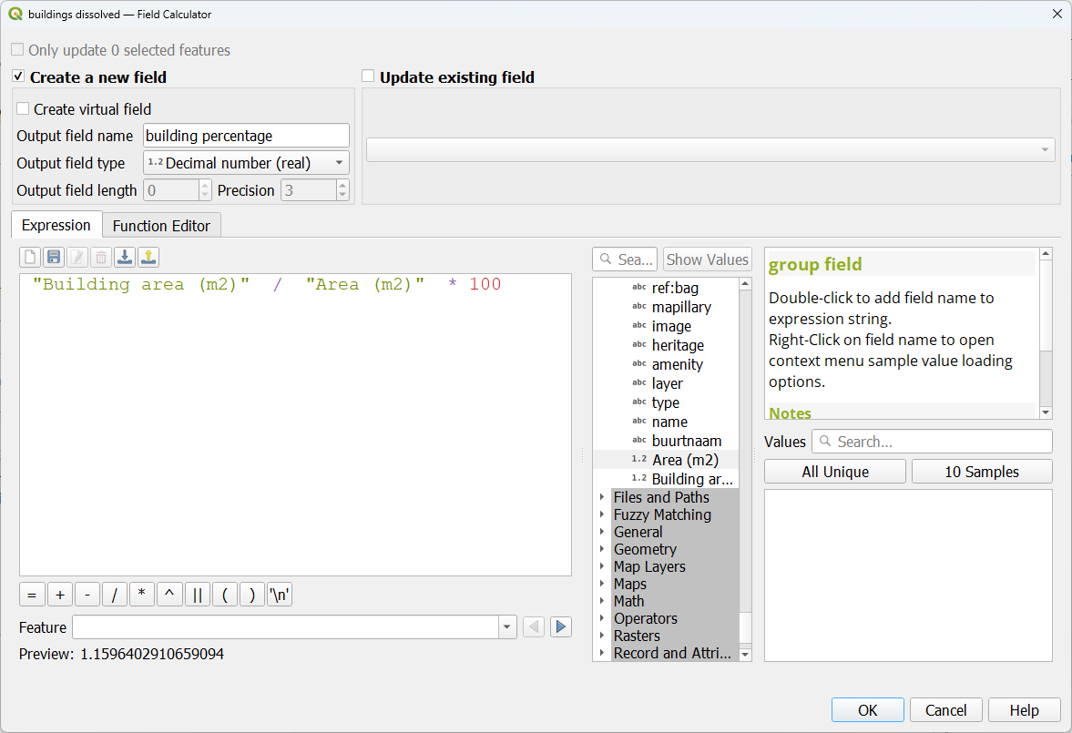
5. Click OK.
6. Toggle off editing mode by clicking  and confirm that you want to save the changes.
7. Check the results.
8. Close the attribute table.
In the next section we'll add the percentages to the neighbourhood layer.
2.5. Join attributes
For visualisation, it is much nicer to give the neighbourhood polygons a gradient for the percentage of building cover. Therefore, we need to join the building percentage field to the neighbourhoods layer. That's not a spatial join, but a join based on a key field in both attribute tables. In this case, the neighbourhood name.
1. In the Layers panel, right-click on the neighbourhoods layer and choose Properties... from the context menu.

2. In the Layer Properties dialog go to the Joins  tab.
tab.
3. Click  to add a new join.
4. In the Add Vector Join dialog, make sure you choose Buildings dissolved as Join layer and buurtnaam for both the Join field and Target field.
5. Expand Joined fields and choose only building percentage, otherwise all fields will be joined.
6. Under Custom field name prefix, delete everything. In that way there will be no prefix for the joined field, which is already clear by itself.

7. Click OK to close this dialog and click again OK to close the Layer Properties dialog.
8. Check the attribute table of the neighbourhoods layer.
In the next section, we'll style the results.
2.6. Style the building densities
Let's style the result.
1. Go to the Layer Styling panel and make sure the neighbourhoods layer is active.
2. Change the renderer to Graduated and choose building percentage as Value.
3. Choose a colour ramp from white to red. Set the Mode to Natural breaks (Jenks) and use 5 classes.
4. Click Classify.

5. Now go to the Labels  tab.
tab.
6. Change it from No labels to Single labels.
7. Choose buurtnaam for Value.
8. Go to the Formatting  tab.
tab.
9. At Wrap on character type a space to split words to different lines for a better fit in the polygons.
10. Evaluate the result.
- Which neigbourhood has the highest density?
- Does the center of Rotterdam has high densities?
- Are there relations between building densities and other attributes in the neighbourhood layer?

Check this video for the steps in this chapter:
3. Spatial metrics
When we look at the scale of a city, we can characterize it using spatial metrics. These are also called landscape metrics or when applied to cities, urban metrics.
In QGIS we can use the LecoS plugin.
1. Install the LecoS plugin from the Plugins Manager.
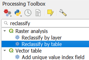
2. Click  to go open the Processing Toolbox panel
3. Expand the LecoS group and then the Landcape statistics group.
In the next section, we'll explore these tools.
3.1. Raster class areas
Let's get a table with the surface areas of each land-use class in our land-use raster.
1. Open the Count Raster Cells tool.

2. In the Count Raster Cells dialog, choose LGN2022_Rotterdam as Raster layer and save the result to your GeoPackage with the table name land use count.

3. Click Run. Click Close when processing is completed.
4. Open the land use count attribute table.
The Value field is the class number that you can find in your land-use layer. Number is the number of pixels.
To get the surface area, we need to multiply the number of pixels with the raster resolution. The resolution is 5 m, so the one pixel is 5 x 5 = 25 m2.
5. Click  to open the Field Calculator. This will automatically toggle to Editing Mode.
6. In the Field Calculator dialog, Create a new field with Area (m2) as the Output field name and Decimal number (real) as Output field type.
Here we can't use $area in the expression, because the table has no geometry. It's just a table, not a vector GIS layer.
7. In the middle panel expand Fields and Values and double-click on Number to add it to the expression. Then click  and type 25 to have the following expression:
"Number" * 25
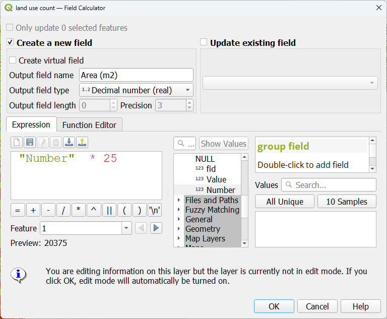
8. Click OK.
9. Click  to toggle off editing mode and confirm that you want to save the edits.
10. Now click on the Area (m2) field name two times so that it sorts the rows from large to small.

- Which are the four largest land-use classes (names) in Rotterdam?
3.2. Reclassify rasters
Our land-use map contains more detail than we need. Let's aggregate classes so it better fits our needs for urban studies.
1. In the Processing Toolbox, go to Raster analysis | Reclassify by table.
2. Choose LGN2022_Rotterdam as Raster layer.
3. Click the browse  button at Reclassification table.
We're going to create a lookup table to end up with the following land-use classes:
- Water bodies
- Urban
- Infrastructure
- Semi-natural
- Agriculture
- Other
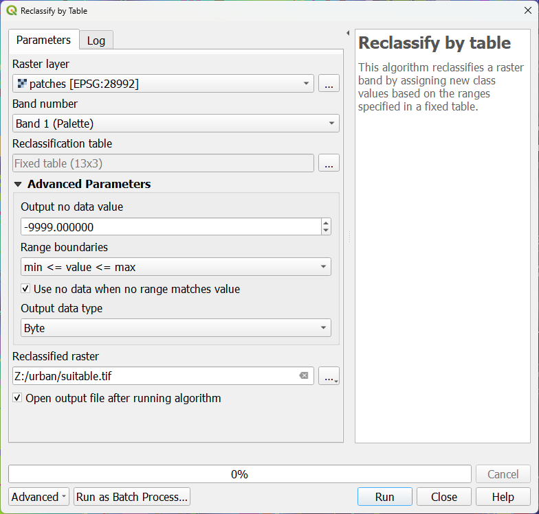
4. Create exactly the lookup table as given below.
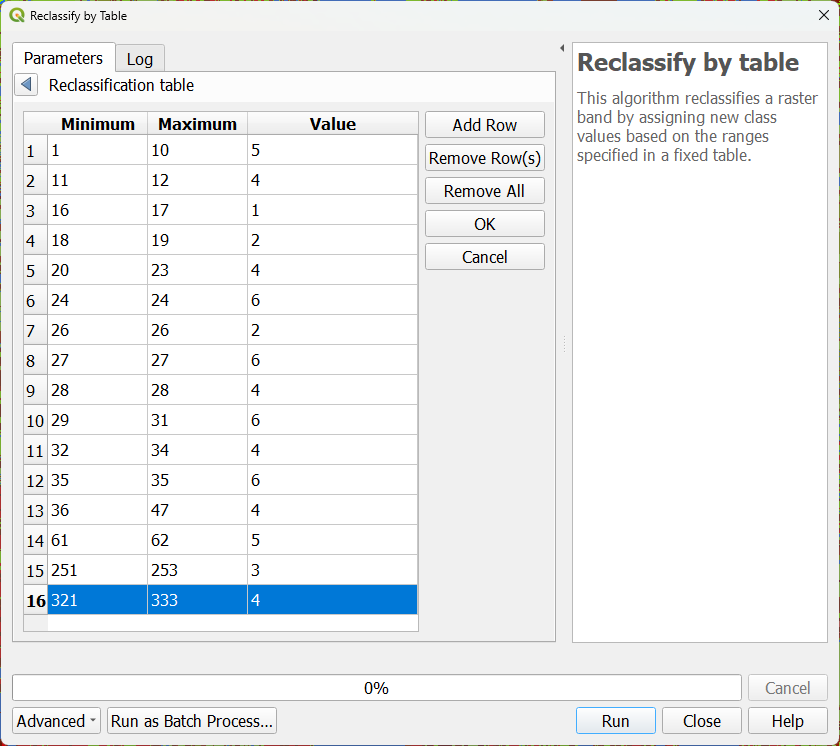
5. Click OK or the blue arrow to go back.
6. Expand the Advanced Parameters section.
7. Change the Range boundaries to min <= value <= max, so it will include both lower and higher boundaries of each defined range in the lookup table.
8. Change the Output data type to Byte. This means that we need 8 bits integers as output, so we can store max 256 values (0 - 255).
9. Save the result to landuse.tif in your project folder.

10. Click Run. Click Close when processing is completed.
- Is the result a boolean, discrete or continuous raster?
- Which renderer should we use to style the raster?
11. Go to the Layer Styling panel. Make sure the landuse layer is active and choose the Paletted/Unique values renderer.
12. Click Classify so each value in the raster gets a unique colour.
13. Modify the colours and class labels so that the raster has intuitive colours and the class names.

Now let's use this aggregated land-use map for analysing spatial metrics at the landscape level.
3.3. Landscape wide statistics
Now let's look at Landscape wide statistics.
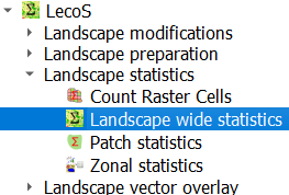
1. In the Processing Toolbox, go to LecoS | Landscape statistics | Landscape wide statistics.
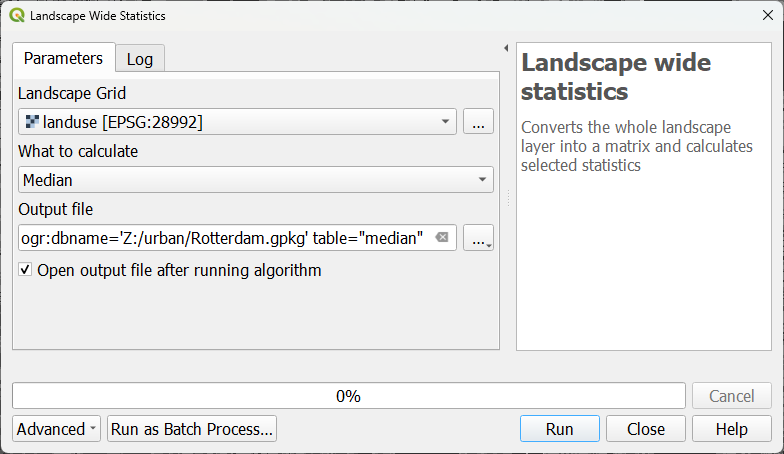
This tool will give you overall statistics for the land-use raster.
Let's calculate the Median land-use class.2. In the Landscape Wide Statistics dialog choose landuse as Landscape Grid. Under What to calculate choose Median. Save the result to your GeoPackage with the table name median.
3. Click Run. Click Close when processing is finished.
4. Open the attribute table of median.
- Which land-use class is the median?
- What does this mean?
Some of the diversity metrics give errors unfortunately.
Let's continue and check out the Patch statistics in the next section.
3.4. Patch statistics
We're going to explore connectivity of green infrastructure in the urban environment.
1. In the Processing Toolbox, go to LecoS | Landscape statistics | Patch statistics.
2. Make sure that landuse is chosen as Landscape Grid.
Type 4 at Choose Landscape Class.
Class 4 is Semi-natural.
We can calculate a lot of different metrics here.
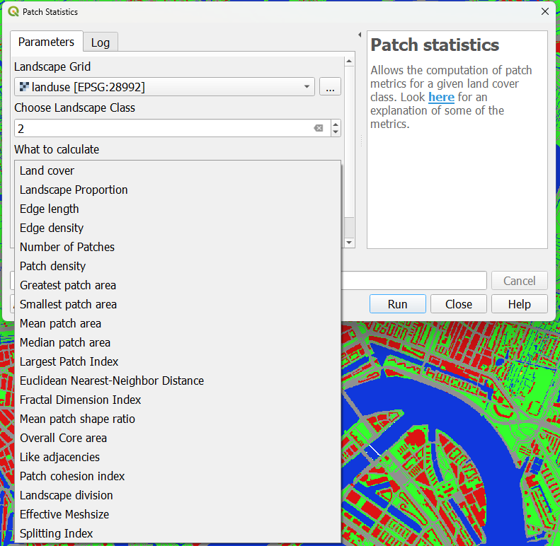
3. Choose Patch cohesion index.
The Patch cohesion index quantifies the physical connectedness of a specific patch type within a landscape. A higher value means that the patches of the class are more connected.
4. Save the output to your GeoPackage with the table name patch cohesion index nature.
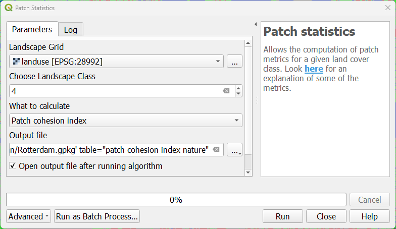
5. Click Run. Click Close after processing is completed. This can take a while.
6. Open the attribute table of patch cohesion index nature and check the result.
This value doesn't say much, unless we compare it with another area or another land-use class.
7. Repeat the calculation for the urban class by yourself. Call the result table patch cohesion index urban.
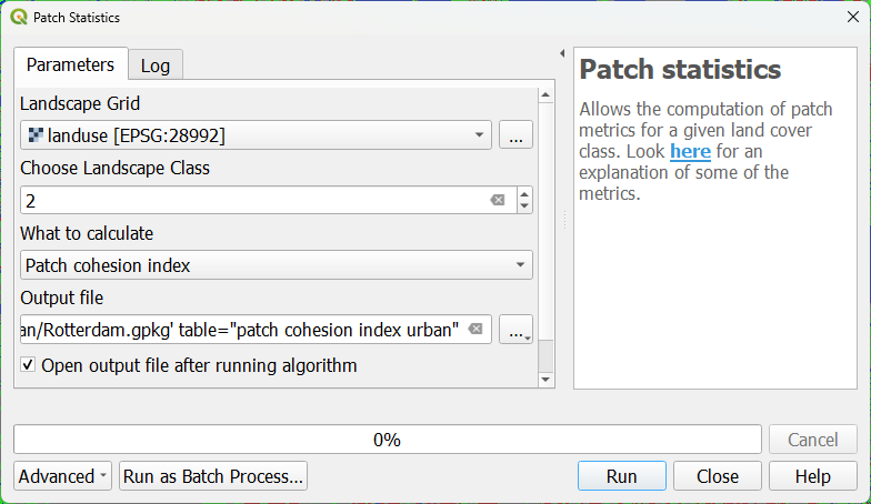
- Which land-use class is more connected? Semi-natural or urban?
- Which land-use class in your raster is most connected if you would make an educated guess?
9. Repeat the steps to calculate the Patch cohesion index for Infrastructure.
- What can you conclude?
You can try other patch-based metrics. Their descriptions can be found here.
This video shows the steps in this chapter:
4. Find locations for climate adaptation measures
In this chapter, we will look for locations to develop climate adaptation measures.
With the land-use map we can identify open spaces in the city and with map algebra we can select patches that are suitable.
4.1. Find open places
- Have a look at the original land-use map (LGN2022_Rotterdam) and check which land-use classes are potentially suitable for developing climate adaptation measures.
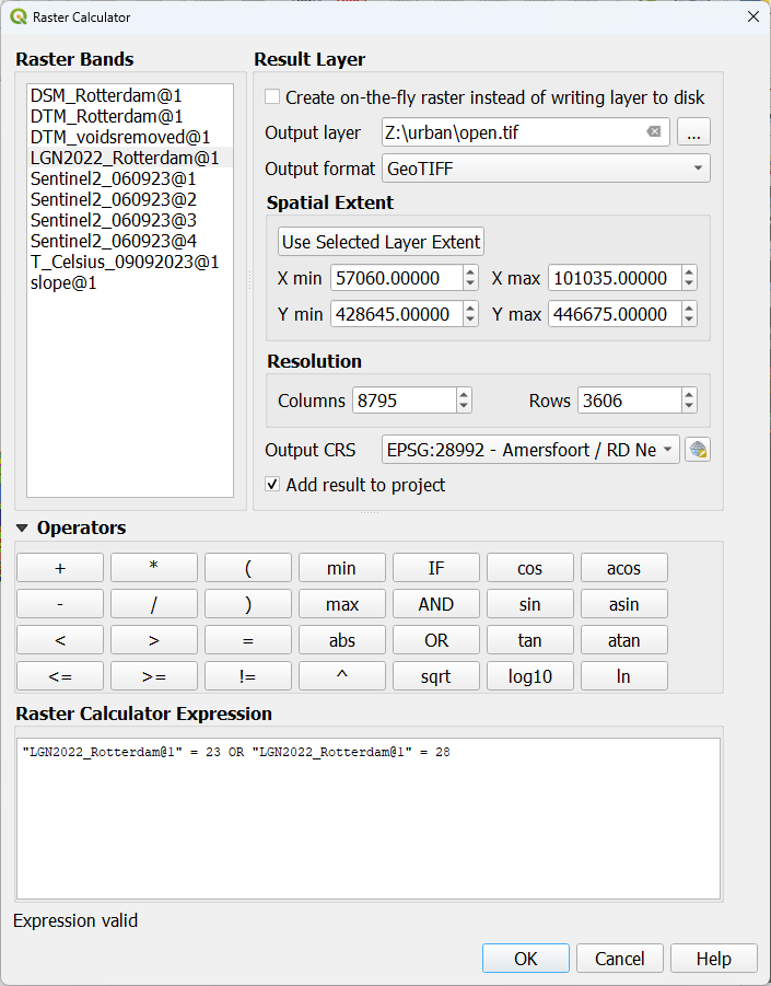
Let's assume that the land-use classes 23 (grass in primary built-up areas) and 28 (grass in secondary built-up areas) are potentially suitable. Let's create a a boolean raster that is true for these classes and false for all other classes. We can do this with the Raster Calculator.
1. In the main menu go to Raster | Raster Calculator....
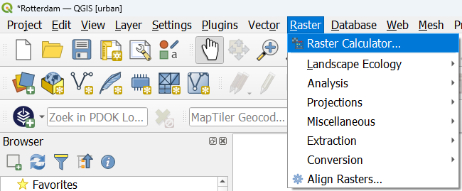
2. Under Raster Bands, double-click on LGN2022_Rotterdam@1 to add it to the expression. Then complete the expression so it states:
"LGN2022_Rotterdam@1" = 23 OR "LGN2022_Rotterdam@1" = 28
Tip: click on the operators instead of typing them.
- Why do we use OR and not AND?
3. Save the result in the project folder and call it open.tif.
4. Click OK.
- The result is a boolean raster. Which renderer do we use to style a boolean raster?
5. Go to the Layer Styling panel and make sure the open layer is active.
6. Use the Paletted/Unique values renderer and click Classify.
7. Change the Color for 0 to red and change the Label to Not open. In the same way, change the Color for 1 to green and change the Label to Open.
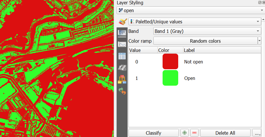
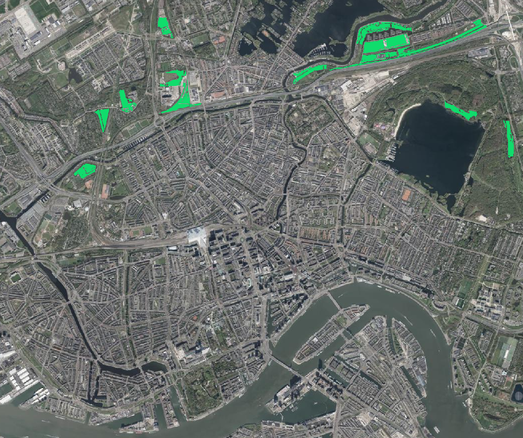
Now we see in green all the open patches in the city (based on our simple assumption).
However, we do not distinguish individual patches. Let's fix that in the next section.
4.2. Set zero to nodata
In the previous section, we have created a boolean raster with True (1) for open spaces and False (0) for other areas. To develop plans, we need to check individual open patches.
Before we can make the patches, we need to remove all False pixels by making them nodata. Then they're not considered as patches.
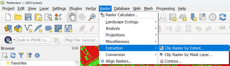
1. In the main menu, go to Raster | Extraction | Clip Raster by Extent....
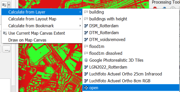
2. In the Clip Raster by Extent dialog, make sure that open is chosen as the Input layer.
3. At Clipping extent, click the arrow to go to the drop-down menu and choose Calculate from Layer | open, so exactly the same extent as the input layer will be used.
4. To make all zeros nodata, set Assign a specified nodata value to output bands to 0.
5. Save the result to open_nodata.tif in your project folder.
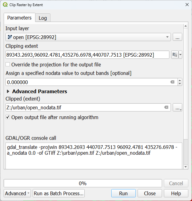
6. Click Run. Click Close after processing has completed.
7. Style the result layer in such a way that all cells with value 1 are green and labelled with Open.
4.3. Create patches with clump
Now we're ready to use the clump operation.
1. Click to open the Processing Toolbox panel.
2. Go to GRASS | Raster (r.*) | r.clump.
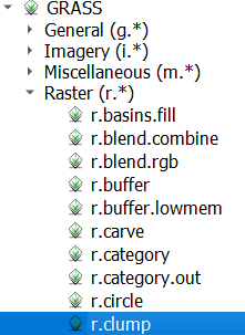
3. In the r.clump dialog, choose open_nodata as Input layer. Type open patches for the Title for output raster map, keep the rest as default and save the result as patches.tif in your project folder.

4. Click Run. Click Close after processing.
Note that now only cells that are horizontally and vertically connected will form a patch. If you want to also use diagonal connections, you need to check the box under the Advanced Parameters section.

Now all the open patches have a unique cell id.

In the next section, we'll have a closer look at the properties of patches.
4.4. Patch areas
Let's check the areas of the patches. We'll use another tool than the one from LecoS, so you can see the difference.
1. In the Processing Toolbox, go to Raster analysis | Raster layer unique values report.
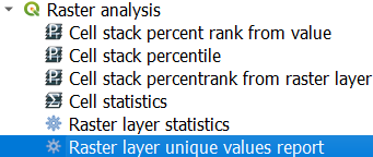
2. In the Raster Layer Unique Values Report dialog, choose patches as Input layer and save the Unique values report to patch_stats.html in your project folder. Also save the Unique values table to your project folder as patch_stats.csv. Make sure you choose Save to file... and change the format to CSV!
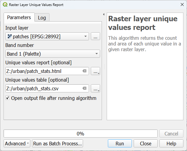
3. Click Run. Click Close after processing is completed.
4. View the results. You can double-click on the Unique values report in the Results Viewer panel. This will show the result in HTML format in your browser.
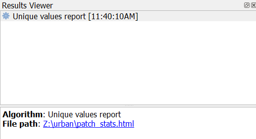
5. The CSV file has been added to your Layers panel. You can open it as an attribute table. You can also open the patch_stats.csv file in notepad using the file explorer. Check the format.
Now we know for each individual patch the surface area in m2. You can use the Field Calculator in the attribute table of patch_stats to select patches that are larger than a certain threshold. Then you can use the Raster Calculator to create a new boolean raster. You can also reclassify the patches. Alternatively, you can also convert them to polygons and use vector processing tools to select the patches that you need. Raster zonal statistics can be used to derive statistics based on another layer.
In another tutorial, we'll use the Raster zonal statistics.
4.5. Proximity analysis
Let's assume that we want to find patches that are close to water bodies. In this section, we'll create a proximity raster and use that for the selection of patches.
1. In the main menu, go to Raster | Analysis | Proximity (Raster Distance)....

2. In the Proximity (Raster Distance) dialog, choose landuse as Input layer and type 1 at A list of pixel values in the source image to be considered target pixels. This is the Water bodies class.
3. Change Distance units to Georeferenced coordinates, so the result raster will have distances in meters.
4. Keep the rest as default and save the result as proximity.tif in your project folder.
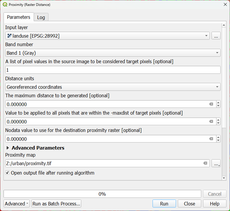
5. Click Run. Click Close after processing.
- Is the result raster boolean, discrete or continuous?
- Which renderer should be used?
6. Go to the Layer Styling panel and make sure the proximity raster is active. Choose Singelband pseudocolor as renderer and choose the Turbo colour ramp.

7. Move the patches layer to the top, so you can see which patches are closer and which are further from surface water.
Now we can use zonal statistics to derive the proximity statistics. Because we have two raster layers, we'll use the Raster layer zonal statistics tool.
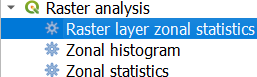
8. In the Processing Toolbox, go to Raster analysis | Raster layer zonal statistics.
9. In the Raster Layer Zonal Statistics dialog, choose proximity as the Input layer and patches as the Zones layer. Save the result to your GeoPackage with the name patch proximity.
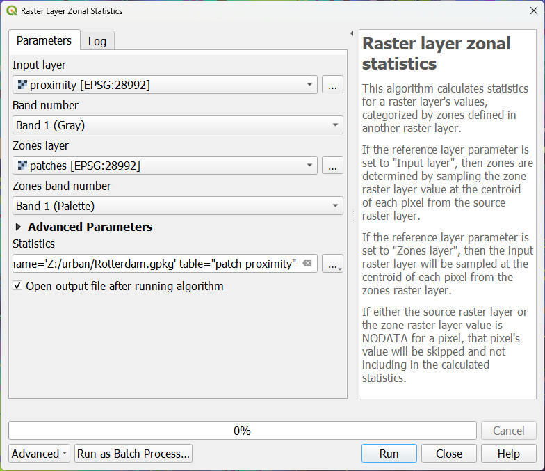
10. Click Run. Click Close after processing has finished.
11. Open the attribute table of patch proximity.
Now we can select the patches that are of a certain minimum size and maximum distance from surface water.
12. In the attribute table, click  to select features by using an expression.
13. Create the following expression:
"m2" > 25000 AND "max" < 100
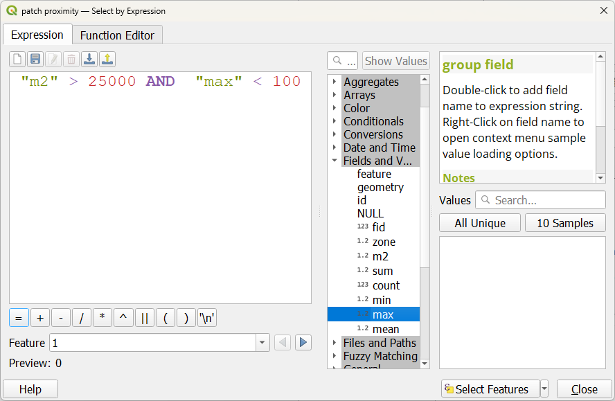
14. Click Select Features. Click Close.
- How many patches are selected?
The zone field shows the patch number.
Now we can make a new raster with only the selected patchs.
15. Use the Reclassify by table tool as we did in Section 3.2. Create a boolean raster with True for the selected features and False for the other features.
Hint: click at the bottom of the attribute table at Show All Features and change it to Show selected features.
5. Conclusion
In this tutorial, you have learned to:
- Calculate areas and densities using polygons.
- Calculate spatial metrics at the landscape and patch level.
- Find potential locations for the development of climate adaptation solutions.
More map algebra in this playlist: