Flood analysis with GIS
| Site: | OpenCourseWare for GIS |
| Course: | Planning for Urban Climate Adaptation |
| Book: | Flood analysis with GIS |
| Printed by: | Guest user |
| Date: | Friday, 19 June 2026, 12:25 PM |
1. Introduction
In this tutorial, we are going to do flood analysis.
We're going to use a digital terrain model (DTM) to create flooded areas. We'll extrude building footprints from OpenStreetMap using the average value in a digital surface model (DSM). With these data, we can find damaged buildings and visualize the flooded areas in 3D.
2. Preprocesssing data
Before we can start our flood analysis, we need to preprocess the datasets. The following preprocessing steps are needed:
- Clip DTM
- Interpolate voids
- Extrude buildings
Let's start with organizing the data.
1. Start QGIS 3.34.
2. Open the project of the first tutorial.
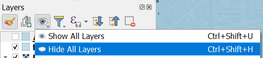
3. Hide all layers.
4. Select the following layers with the Control key pressed:
- buildings
- DTM_Rotterdam
- DSM_Rotterdam
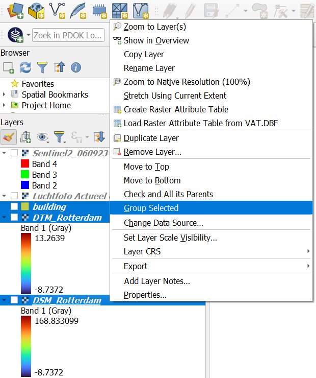
6. Name the group Flood analysis and drag the group to the top.
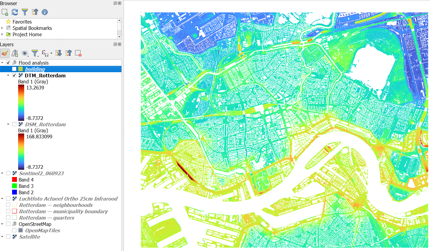
2.1. Interpolate voids
The DTM has all the objects, like buildings, filtered out of the raster. This results in voids: nodata pixels. To also get the terrain elevation of the locations of buildings, we'll interpolate the voids.1. Make sure to make DTM_Rotterdam visible by checking the box in the Layers panel.
2. In the toolbar, click
 to open the Processing Toolbox panel.
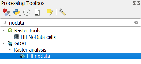
3. In the processing toolbox, search nodata.
4. Double-click on the GDAL | Raster analysis | Fill nodata tool.
5. In the Fill nodata dialog, choose for Input layer DTM_Rotterdam. Only change the Maximum distance (in pixels) to search out for values to interpolate to 100. 100 pixels of 0.5 m equals 50 meters, which should be enough to interpolate voids of buildings.
6. Call the output Filled layer DTM_voidsremoved.tif.
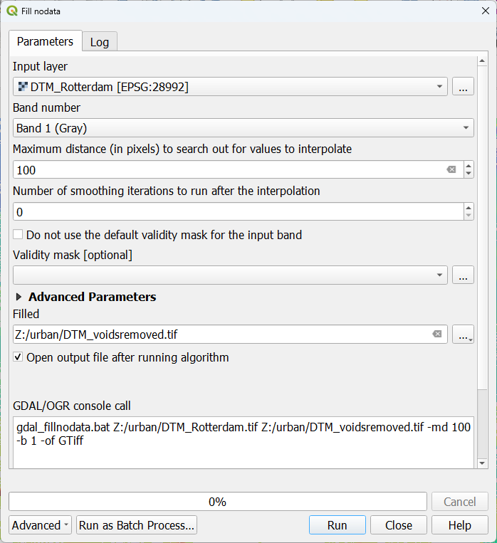
7. Click Run. Click Close when processing has finished.
8. Drag the DTM_voidsremoved layer into the Flood analysis group and style the layer with the same colour ramp as the original layer.
9. Go to the histogram tab
 .
.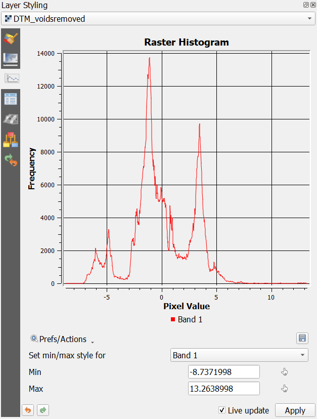
- What can you tell about the minimum and maximum elevations?
- Can you explain the peaks?
To better interpret this urban landscape, we're going to calculate the slopes.
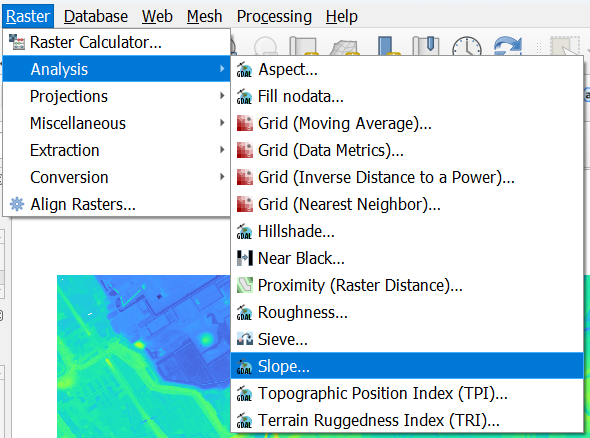
10. In the main menu, go to Raster | Analysis | Slope....
11. In the Slope dialog, make sure the DTM_voidsremoved layer is chosen as the Input layer. Keep the rest as default and save the result to slope.tif in the folder of your GeoPackage.
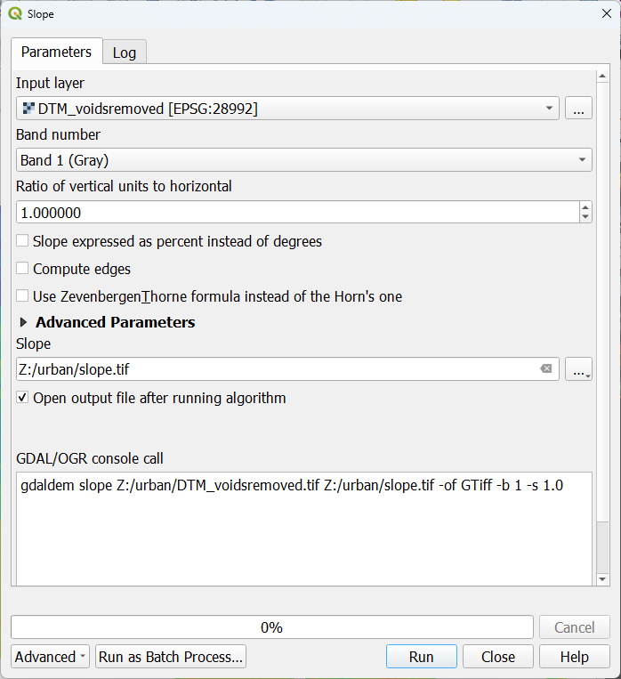
12. Click Run. Click Close when processing is completed.
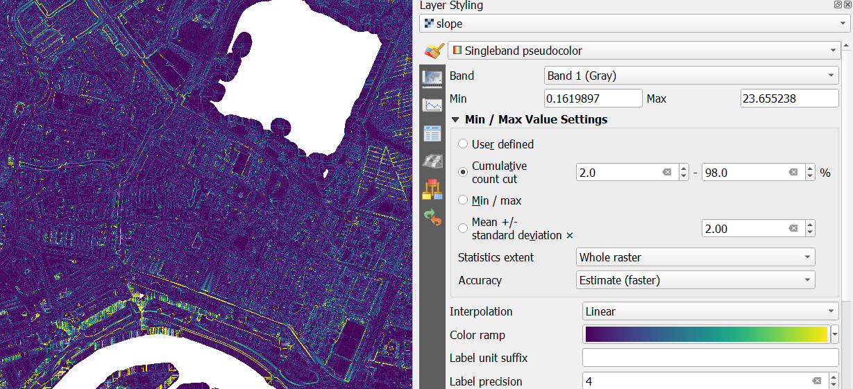
13. Drag the slope layer into the Flood analysis group and style the layer with a ramp.
14. Check the histogram.
- What do you observe?
- What are most of the steep slopes in this city?
15. Because many pixels have a low slope and few have a high slope, you can best change the Min / Max Value Settings to Cumulative count cut, to see more details
Now you can clearly see the dykes and highway ramps.
Next, we're going to work on the building heights.
2.2. Extrude buildings
The buildings that we've downloaded from OpenStreetMap have attributes that we can use for their height:
- height
- building:levels, which is the amount of floors
Not all buildings have these values and the values are sometimes noted with their units. This makes it a lot of work to clean up the data.
Therefore, here we're going to use the elevation from the DSM to add the Z attribute to the building polygons.
1. In the Processing Toolbox open the tool Raster analysis | Zonal statistics.

2. In the Zonal Statistics dialog, choose the buildings layer as Input layer and DSM_Rotterdam as Raster layer. Type for Output column prefix Z_, so the field will be easy to recognize. For Statistics to calculate only choose the Mean. In that way each building polygon will get the mean value from the overlapping pixels in DSM_Rotterdam. Save the result in the existing GeoPackage with the name buildings with height.
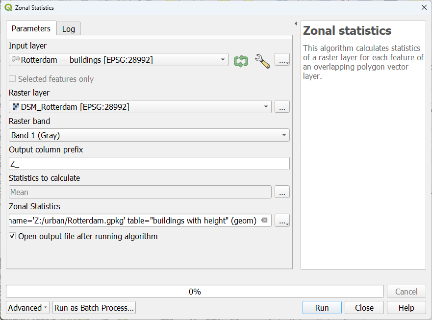
3. Click Run. Click Close after processing has completed.
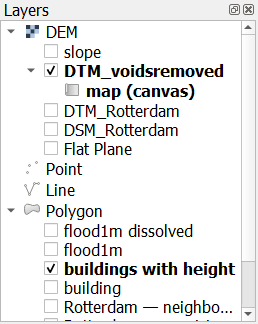
4. Make sure that in the Layers panel, this layer is at the top of the Flood analysis group and that below the DTM_voidsremoved layer is visible.
Now let's check the result in the QGIS 3D View.
5. Save the project.
6. Go to the Layer Styling panel and make sure that the buildings with height layer is active.
7. There go to the 3D View  tab where we can set the 3D visualization properties.
8. Set the renderer to Single Symbol.
9. At Extrusion, click  to set a data-defined override.
10. Select Field type and choose the Z_Mean field.
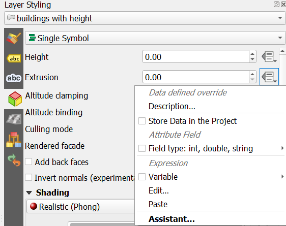
11. Make sure that the other settings are the same as in this screenshot:
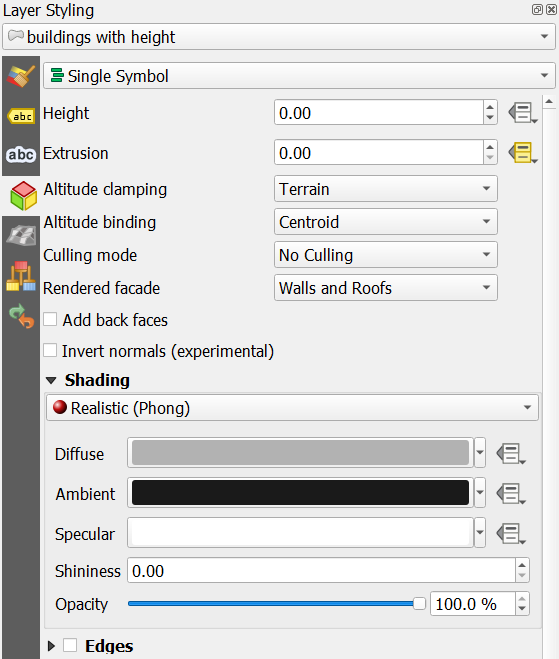
Now we're ready to check our buildings in 3D.
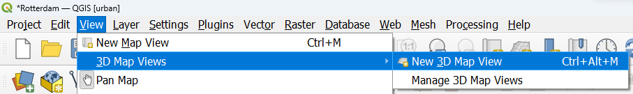
12. From the main menu, select View | 3D Map Views | New 3D Map View.
13. In the new 3D map view, click  and choose Configure....
14. In the Terrain tab change Type to DEM (Raster Layer) and choose DTM_voidsremoved for Elevation. In this way the DTM elevation values will be used to visualize the DTM. The buildings will be shown on top. Change the Tile resolution to 512 px to see more detail.
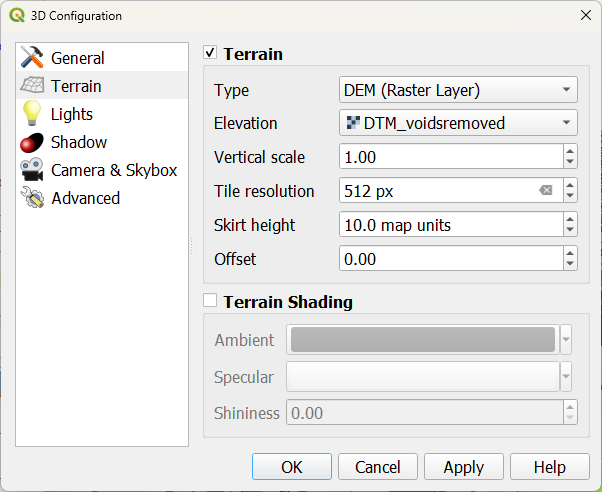
15. Click OK.
Wait until the 3D view renders.

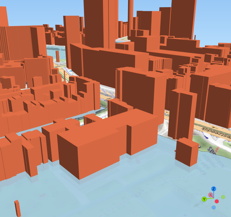
Now we can see the 3D buildings on top of the terrain.
3. Prepare flood extent layers
In this chapter, we're going to prepare the flood extent layers. We'll use the DTM and the QGIS Raster Calculator.
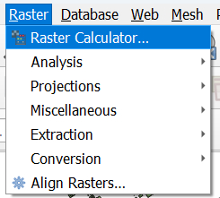
1. In the main menu, go to Raster | Raster Calculator....
In the Raster Calculator, you can see all raster layers under Raster Bands. The @# shows the band number. Our DTM and DSM layers are singleband raster layers, so they all show @1. For the Sentinel2 you can see that the different bands are showns (@1, @2, etc.).
2. At Raster Bands, double-click on DTM_voidsremoved@1 to add it to the Raster Calculator Expression. Then click <= and type 1.
In this way you have composed the expression:
"DTM_voidsremoved@1" <= 1
which means that all pixels of DTM_voidsremoved that have a value less than or equal to one will result in boolean true (one) and other pixels will have boolean false (zero).
3. Under Result Layer use  to browse to your project folder and save the result to flood1m.tif.

4. Keep the rest as default and click OK.
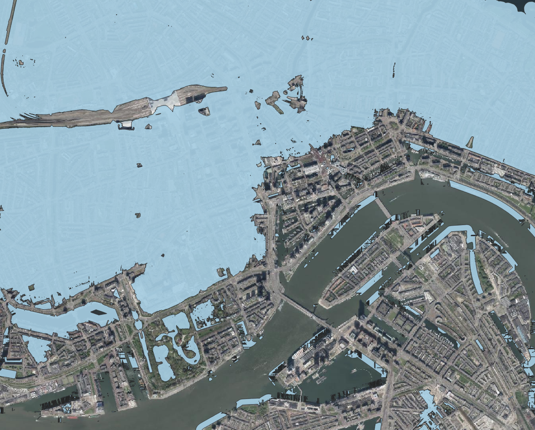
5. Visualize the result. For boolean rasters we use the Paletted/Unique values renderer. Remove the zeros, so they're transparent. Make the ones blue, so we can clearly see the flood extent over our other layers.
It's nicer to visualise the flood extent as a vector layer. Let's convert the raster to vector.
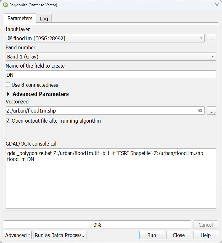
6. In the main menu, go to Raster | Conversions | Polygonize (Raster to Vector)....

7. In the Polygonize dialog, choose flood1m as the Input layer. Keep the rest as default and save the result as a shapefile with the name flood1m.shp.
8. Click Run. Click Close after processing has completed.
As you can see, the polygon has both the flooded and not flooded areas. Let's remove the latter.
9. In the Layers panel, go to the attribute table of the flood1m vector layer.
10. Click  to select features with an expression.
11. In the Select by Expression dialog, go to the middle panel, expand Fields and Values and double-click on the DN field to add it to the expression. Then click  and type 1.
Now your expression should look like this:
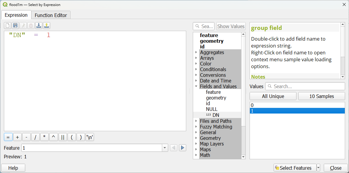
12. Click Select Features and click Close to close the dialog.
In fact we want to delete the zeros, so we need to invert the selection (or go back and choose "DN" = 0).
13. Click  to invert the selection.
Now all the features with value 0 for DN are selected.
14. Click  to toggle to editing mode.
15. Click  to delete these features.
16. Click again to toggle off editing mode and confirm that you want to save the changes.
17. Style the polygons with a light blue colour and some transparency.

17. Now repeat this for different flood levels: 0.5, 1.5, 2 m.
4. Find damaged buildings
Now we have layers showing the flood extent, we can use it to select the affected buildings.
1. In the main menu, go to Vector | Research Tools | Select by Location....

2. In the Select by Location dialog, choose to Select features from buildings with height Where features overlap By comparing to the features from flood1m. Select Modify selection by creating new selection.
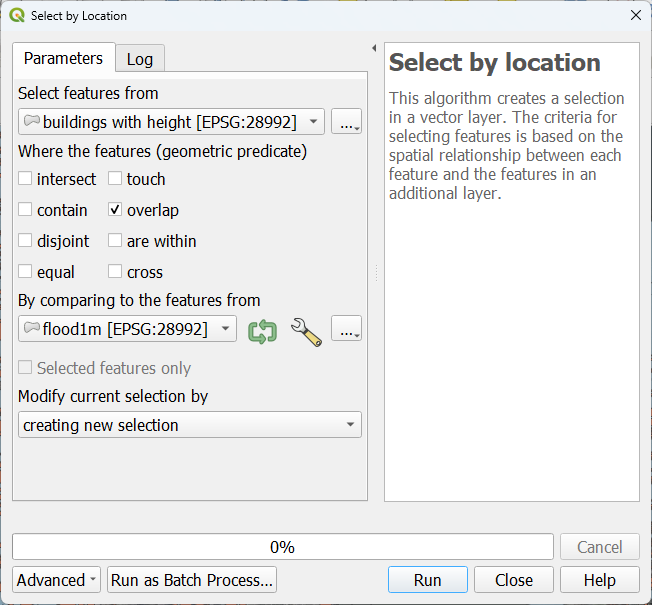
3. Click Run. Click Close after processing is completed.
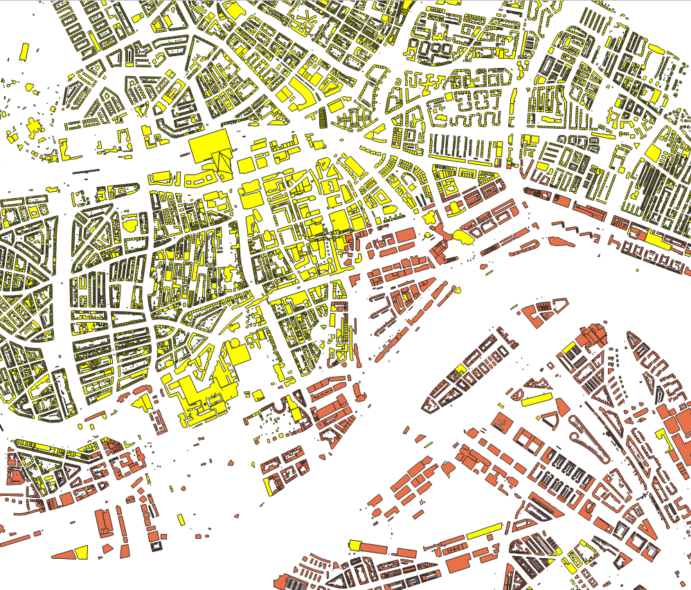
Now you'll see in yellow the selected buildings in the map canvas. These are the buildings affected when the water table rises to 1 m above sea level.
5. Visualize the flood in 3D
A much more intuitive way to look at the affected areas is in 3D.
This time, we're not going to use the native 3D View, but instead we'll use the Qgis2threejs plugin.
1. Install the Qgis2threejs plugin.
2. In the Layers panel, hide all layers.
3. From the Browser panel add XYZ Tiles | OpenStreetMap to the map canvas.
We'll use that as a back drop in the 3D scene.
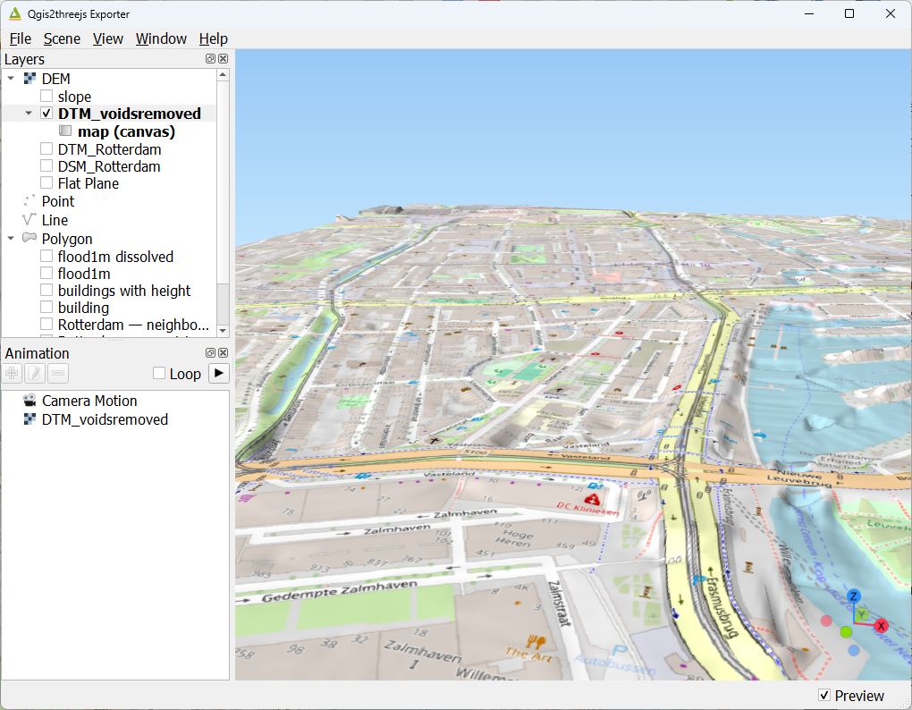
4. Click  to open the plugin window.
5. Under Layers go to DEM and show DTM_voidsremoved by clicking the box.
Now you see the area in 3D. However, the elevation needs some exaggeration.
6. In the menu go to Scene | Scene Settings....

7. In the Scene Settings dialog, increase the Z exaggeration to 3. Keep the rest as default.
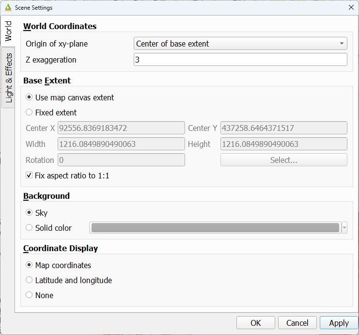
8. Click OK to close the dialog.
Now we can see more relief, but the level of detail is not sufficient.
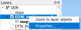
9. Right-click on DTM_voidsremoved and choose Properties... from the context menu.
10. In the Layer Properties dialog increase the Resampling level to the maximum (6). Also increase the Image width to 4096 pixels.
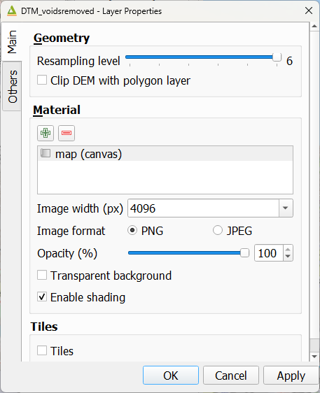
11. Click OK to close the dialog.
If your computer can't handle this, reduce the image width.
Now we can see the relief in more detail. We can see the dykes in the city.
Let's add the buildings.
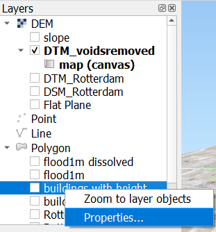
12. Under Layers, right-click on buildings with height and choose Properties... from the context menu.
13. In the Layer Properties, change the Type to Extruded. For Z coordinate, choose the Mode Relative to "DTM_voidsremoved" layer. Under Geometry, set the Height to the Z_mean attribute.
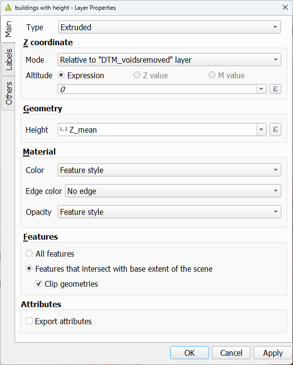
14. Click OK.
15. Check the box to show the buildings with height layer.
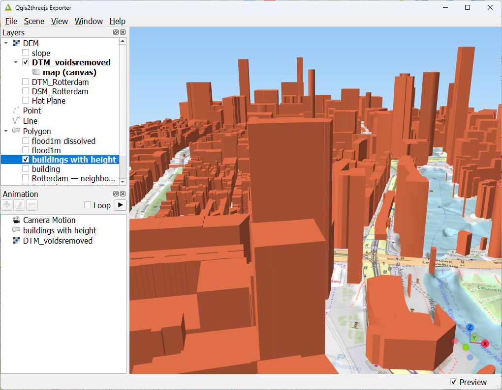
Now let's add a flood extent layer.
16. Under Layers, right-click on flood1m and choose Properties... from the context menu.

17. In the Layer Properties, set Type to Extruded, Z coordinate to Absolute and choose the DN field under Expression. Under Geometry choose also the DN field for Height.

18. Click OK.
- Explore the results.
- Change settings to see the effect.