Tutorial: WaPLUGIN User Interface
| Site: | OpenCourseWare for GIS |
| Course: | Enhancing Water Productivity with WaPOR: A Hands-On Workshop Using WaPLUGIN in QGIS |
| Book: | Tutorial: WaPLUGIN User Interface |
| Printed by: | Guest user |
| Date: | Saturday, 20 June 2026, 3:13 AM |
1. Introduction
WaPLUGIN provides a user-friendly interface that allows users to easily and quickly access WaPOR datasets directly within QGIS projects.
In the next chapters, you'll learn how to sign in and use the different tabs in the interface.
2. Sign In Tab
Only necessary if you need to Access WaPOR V2 Datasets
You need a personal API Token to access WaPOR V2 datasets.
1. Start QGIS Desktop
2. In the Toolbar, click on the WaPLUGIN icon
 . to open the dialog.
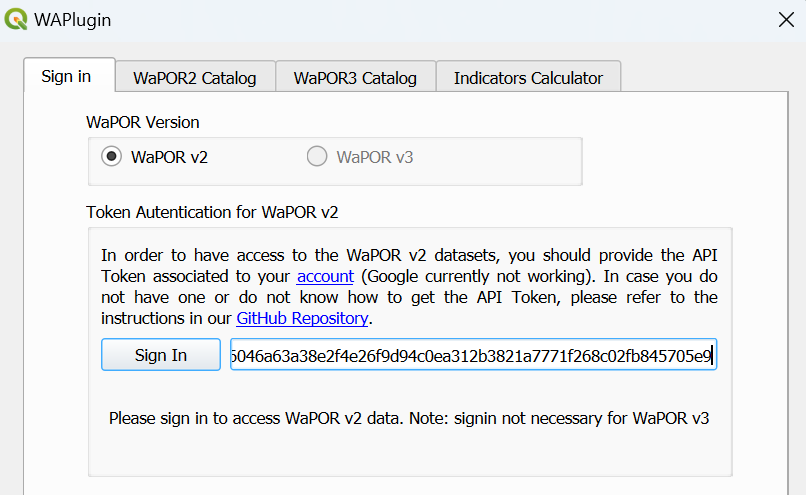
3. At the Sign in tab, navigate to the WaPOR V2 website by clicking the account link .
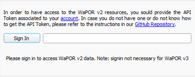
Although the WaPOR v2 data is depricated, you can still access it.
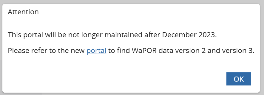
4. Click OK to proceed.
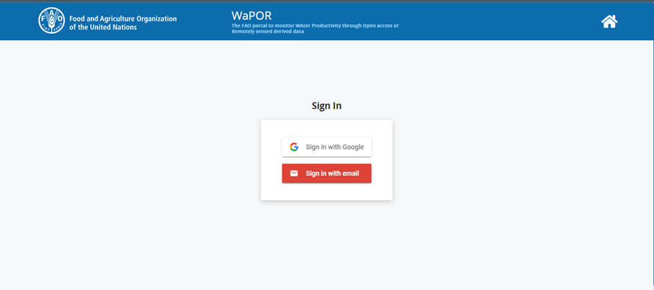
5. If you don’t have an account, register using a non-Google email (Google login is no longer supported on this site).
6. Once your account is created, log in and go to the My WaPOR section by clicking the
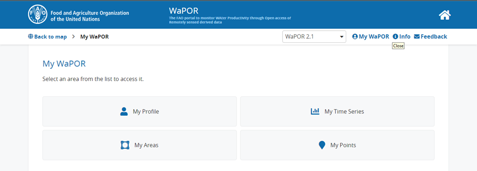
7. Click on My Profile, scroll down, and generate your API Token.
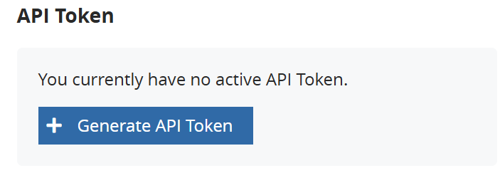
8. Copy and paste your API Token into the designated field in the WaPLUGIN Sign in tab.
Note :
- To save time in future sessions, click “Save Token”. This will store your token, and next time you use WaPLUGIN, you can simply click "Load Token" for automatic sign-in.
- The API sign-in process is only required for WaPOR V2 data. For WaPOR V3, there’s no need for an API Token. You can directly access the WaPOR3 Catalogue Tab.
- Since the workshop will focus on WaPOR V3 datasets, you can skip the API sign-in process.
- If you face any issues or need access to WaPOR V2, feel free to contact us for assistance.
3. WaPOR2 Catalog Tab
In this chapter we will explore the WaPOR2 Catalog tab of the WaPLUGIN.
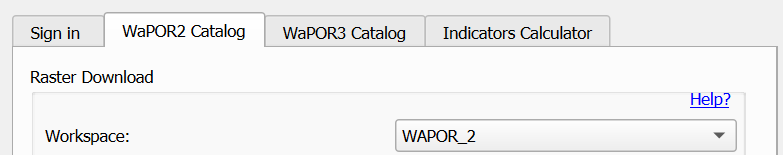
1. Go to the WaPOR2 Catalog Tab in the WaPLUGIN.

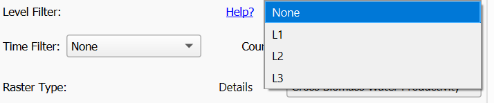
2. Select the workspace from the dropdown menu and choose WaPOR_ 2 (note that other datasets are available but not relevant for this workshop).
- L1: Continental
- L2: National
- L3: Sub-national
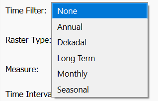
4. Apply the time filter to select the time step, choosing between daily, dekadal, monthly, seasonal, or annual data.
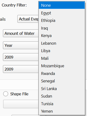
5. Optionally, filter by Country using the dropdown menu, which provides a list of WaPOR V2 partner countries (Not all filters need to be applied simultaneously). This filter only works for Level 3 data.
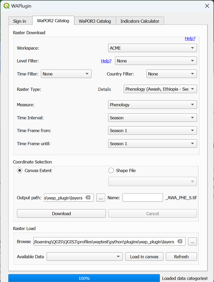
6. Select the Raster Type from the dropdown menu, displaying the available layers based on your previous selections.
7. Use the Details button next to the Raster Type dropdown to view a full description of the dataset, including conversion factors required for correcting downloaded data. (More detailed information is available in the FAO WaPOR Database Methodology Report.)
8. Define the Time Frame by selecting the start and end dates for the raster download. The buttons will be automatically populated once the layer type or time filter is selected (Download multiple rasters at once).
9. Define the spatial extent of your raster download using one of the following options:
- Canvas Extent: Limit the extent to the visible QGIS map canvas area.
- Shapefile: Use the dropdown to select a shapefile from your project and clip the data accordingly. (For L3 data, ensure the map canvas is zoomed in on the study area or country of interest. It’s recommended to use the QuickMapServices plugin to easily access basemaps and locate your study area.)
10. If needed, you can change the output path using the Output Path option.
By default, the downloaded data will be saved as [Name] [level] [place] [raster type] [time filter].tif. The [Name] can be customized by the user.
11. After setting the necessary parameters, click the Download button.
12. Monitor the progress bar to track the status of your raster download.
13. Once the download is complete, navigate to the Raster Load Section to load the downloaded data into QGIS.
14.The folder containing the downloaded data is automatically set to the path of the layers folder created by the plugin.
15. In the Available Data dropdown menu, select the rasters you want to load into the QGIS map canvas.
16. Click the Load in Canvas button to display the selected rasters in the map canvas (Use the Refresh button to update the list when new datasets are downloaded.)

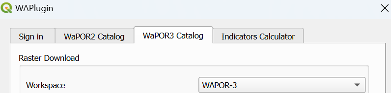
4. WaPOR3 Catalog Tab
In this chapter, we'll guide you through the WaPOR3 Catalog tab of the WaPLUGIN.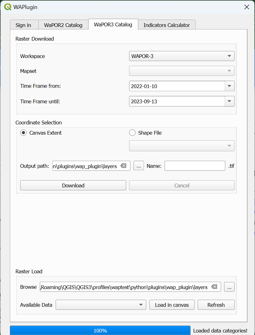
1. Go to the WaPOR3 Catalogue tab in the WaPLUGIN. Note that no API token is required to access the WaPOR3 data (unlike WaPOR V2).
2. Set the Workspace to WAPOR-3.
- Level: Choose from Global, National, or Sub-national.
- Time Scale: Select between Dekadal, Monthly, Annual, or Daily.
- Resolution: Choose the resolution (300m, 100m, 20m) depending on your study area and data needs.

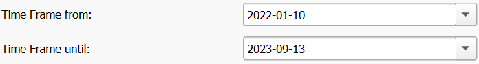
- Click the Time Frame From and Time Frame Until buttons to select the start and end dates.

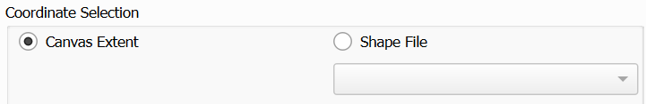
- Canvas Extent: This option limits the download to the visible area in the QGIS map canvas.
- Shapefile: Use the dropdown menu to select a shapefile from your project and clip the raster data to your area of interest (For L3 data, ensure that the map canvas is zoomed in on the study area or country of interest. It’s recommended to use the QuickMapServices plugin to easily access basemaps and locate your study area).
By default, the downloaded data will be saved as [Name] [level] [place] [raster type] [time filter].tif. You can customize the [Name].

7. After setting the necessary parameters, click the Download button. The progress bar will display the download status.
9. Once the download is complete, go to the Raster Load Section to load the data into QGIS.
The plugin will automatically set the folder path to the layers folder where the downloaded data is stored.
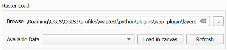
10. In the Available Data dropdown menu, select the raster(s) you wish to load into the QGIS canvas. Click the Load in Canvas button to display the rasters on the QGIS map canvas.
11. If you download additional datasets, use the Refresh button to update the list of available rasters.
Now you've downloaded the data, you can proceed with analysis in the map canvas or use the Indicators Calculator tab, which is explained in the next chapter.
5. Indicators Calculator Tab
In this chapter we'll explore the Indicators Calculator tab of the WaPLUGIN. With this feature you can calculate irrigation performance indicators.1. Open the Indicators Calculator tab in the WaPLUGIN.

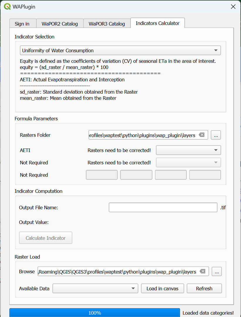
2. Select the desired irrigation performance indicator from the dropdown menu under Indicator Selection.
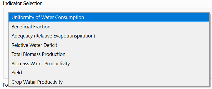
There are currently 8 available indicators:
- Uniformity of Water Consumption
- Beneficial Fraction
- Adequacy
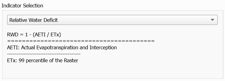
- Relative Water Deficit
- Total Biomass Production
- Biomass Water Productivity
- Yield
- Crop Water Productivity

After selecting an indicator, details about the equation and datasets required for that specific indicator will be displayed.

- The required rasters should be placed in the same folder. This folder is automatically set to the layers folder created by WaPLUGIN when data was downloaded.
- These fields are automatically populated based on the needed raster types.
- Conversion factors are only required for data downloaded from the WaPOR2 Catalogue. You can retrieve these factors by clicking the Details button next to the Raster Type in the WaPOR2 Catalog tab.
- For WaPOR3 Catalogue data, no manual correction is needed as the data is automatically corrected during download.
- For example, users may need prior knowledge about the irrigation schemes or crop types in the study area.
- This raster file will be saved in the same folder as the input rasters once the Calculate Indicator button is clicked.
After computation, the output raster can be loaded into the QGIS map canvas for further analysis.
9. Use the Raster Load Section in the Indicators Calculator tab to load the indicator rasters into QGIS. Simply select the computed indicator and click Load in Canvas.
Using External Rasters
If you want to load a raster from another source (not downloaded via the plugin) and use it as an input parameter to compute the indicators, please ensure the raster file follows the naming structure:
[Name] [level] [place] [raster type] [time filter].tifThis naming convention allows WaPLUGIN to detect and use the raster for computations.