Tutorial: Irrigation Performance Indicators and Water Productivity
| Site: | OpenCourseWare for GIS |
| Course: | Enhancing Water Productivity with WaPOR: A Hands-On Workshop Using WaPLUGIN in QGIS |
| Book: | Tutorial: Irrigation Performance Indicators and Water Productivity |
| Printed by: | Guest user |
| Date: | Saturday, 20 June 2026, 3:13 AM |
1. Introduction
In this tutorial, you will follow a step-by-step guide to download WaPOR datasets and compute various irrigation performance and water productivity indicators using WaPLUGIN.
2. Loading the Study Area Boundary
We'll start with loading the polygon of the study area in QGIS.
1. Download the shapefile provided for the tutorial, which represents an agricultural plot in Oued Hellal, Sudan. Unzip the file in a folder on your hard drive.
2. Start QGIS Desktop.
3. Load the shapefile into your project. There are two ways:
- Go to main menu and choose Layer | Add Layer | Add Vector Layer and select the shapefile.
- Locate the shapefile in the Browser panel and drag it to the map canvas.
To have some more context of the study area, we'll add a satellite image as a base map. We'll use the QuickMapServices plugin.
4. Install the QuickMapServices plugin: in the main menu, go to Plugins | Manage and Install Plugins, search for QuickMapServices, and install it.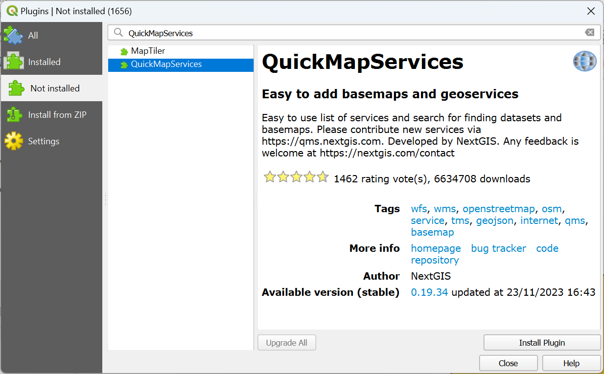
Next, we need to configure access to additional services, because the Google Satellite image is not available by default.
5. In the main menu, go to Web | QuickMapServices | Settings.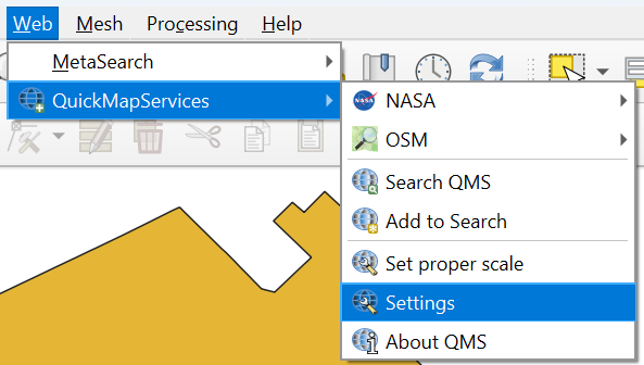
6. In the QuickMapServices dialog go to the More services tab and click the Get contributed pack button.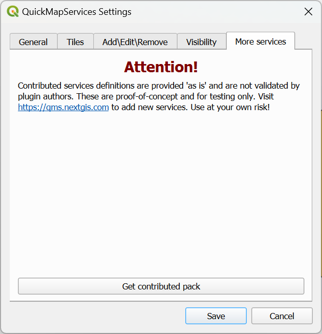
7. Click OK in the popup and Save to close the dialog.
8. Now add the Google Satellite by choosing from the main menu Web | QuickMapServices | Google | Google Satellite.
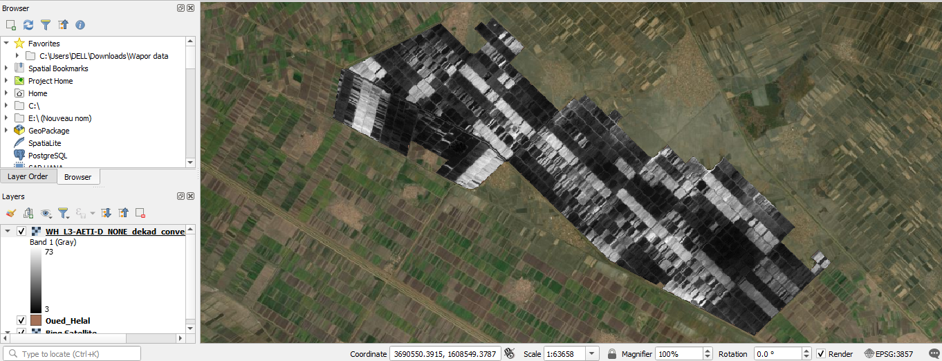
It's better to show only the boundary, so we can see the parcels on the satellite image.
9. In the Layers panel select the Oued Helal layer and click  to open the Layer Styling panel.
10. In the Layer Styling panel click on Simple Fill and change the Symbol layer type to Outline: Simple Line. Change the colour to red and make the line a little thicker.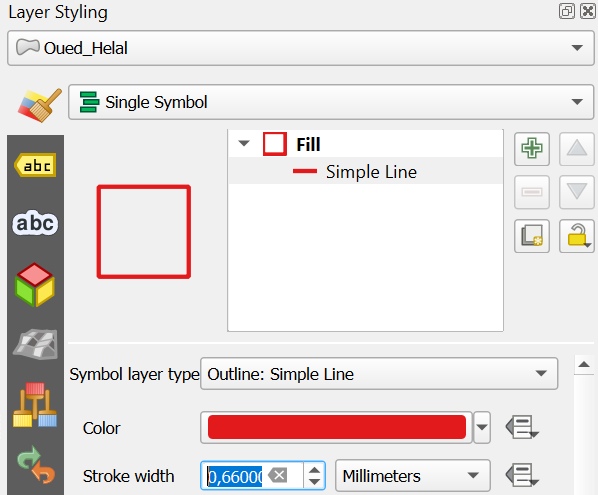
Now you can see the study area.
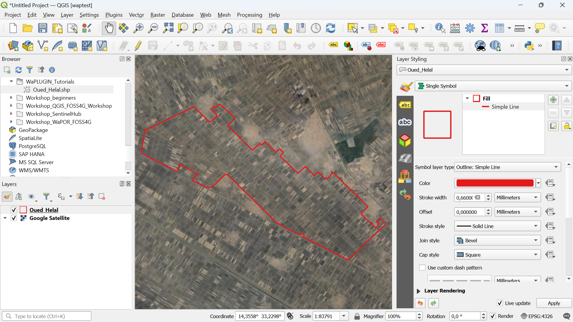
Now we can proceed with downloading WaPOR data for this area using the WaPLUGIN.
3. Accessing WaPOR V3 Data
Now we have loaded the study area polygon in the QGIS map canvas, we can proceed with downloading WaPOR data with the WaPLUGIN.
1. Open the WaPLUGIN dialog from the main menu (Plugins | WAPlugin | Water Accounting and Productivity Plugin) or by using the  icon in the toolbar.
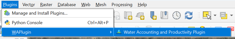
2. Go to the WaPOR3 Catalog tab.
3. In the Workspace dropdown, select WAPOR-3.
For this tutorial, you will need to download the following three datasets:
- Actual Evapotranspiration and Interception (AETI)
- Transpiration (T)
- Net Primary Production (NPP)
Since the Oued Hellal region has Level 3 data available at 20m resolution, select Level 3 (20m) for the highest resolution and we'll use Dekadal data.
Most agricultural plots have a start and end season that varies by region and crop. For this tutorial use:
- Start of season: 01 October 2022
- End of season: 30 April 2023
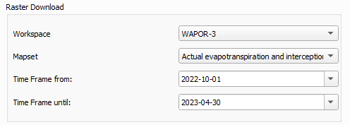
4. In the Mapset dropdown, select Actual Evapotranspiration and Interception (dekadal - 20m).
5. Set the time frame for the season:
- Time Frame From: 01 October 2022
- Time Frame Until: 30 April 2023
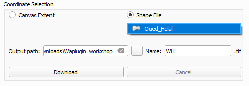
6. In the Coordinate Selection section, choose Shape File.
- From the dropdown, select the vector file corresponding to your study area (Oued_Hellal).
7. Change the output path to a new folder on your computer (e.g., Waplugin_workshop).
8. Add a prefix to the layer name for organization (e.g., “WH” for Oued Helal).
9. Click on Download and wait for the progress bar to complete.
- Since the study area is small, the download time should be short.
- Note: The larger the study area or higher the resolution (L3), the longer the download will take.
9. To verify the download, go to the Raster Load Section.
10. Change the Raster Load path to the Waplugin_workshop folder you created earlier.
11. Click Refresh, and all downloaded layers should appear in the dropdown menu at Available Data.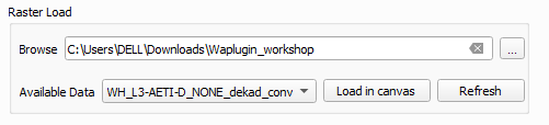
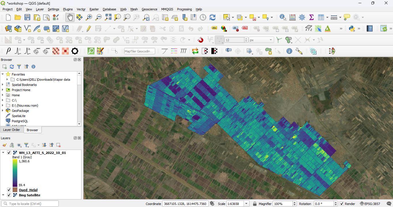
12. To visualize one of the downloaded layers, select it from the dropdown and click Load in Canvas.
- The raster layer will now display in your project canvas.
13. Repeat the same procedure for downloading the Transpiration and Net Primary Production (NPP) rasters:
- Go back to the WaPOR V3 Catalogue tab and select Transpiration (dekadal - 20m) and Net Primary Production (dekadal - 20m) from the Mapset dropdown.
- Use the same time frame, coordinate selection (using the Oued-Helal shapefile), and output path (Waplugin_workshop).
Now we've downloaded all necessary data, we'll aggregate it to seasonal data.
4. Aggregating Dekadal Rasters to Create Seasonal Maps
Seasonal maps are created by summing the dekadal data over the entire season. This feature is currently being developed to be included in the plugin. For this tutorial, we will use the r.series tool available in the QGIS toolbox.
1. Close the plugin dialog and click in the Toolbar to open the Processing Toolbox panel.
2. In the search bar of the toolbox, type r.series to find the tool.
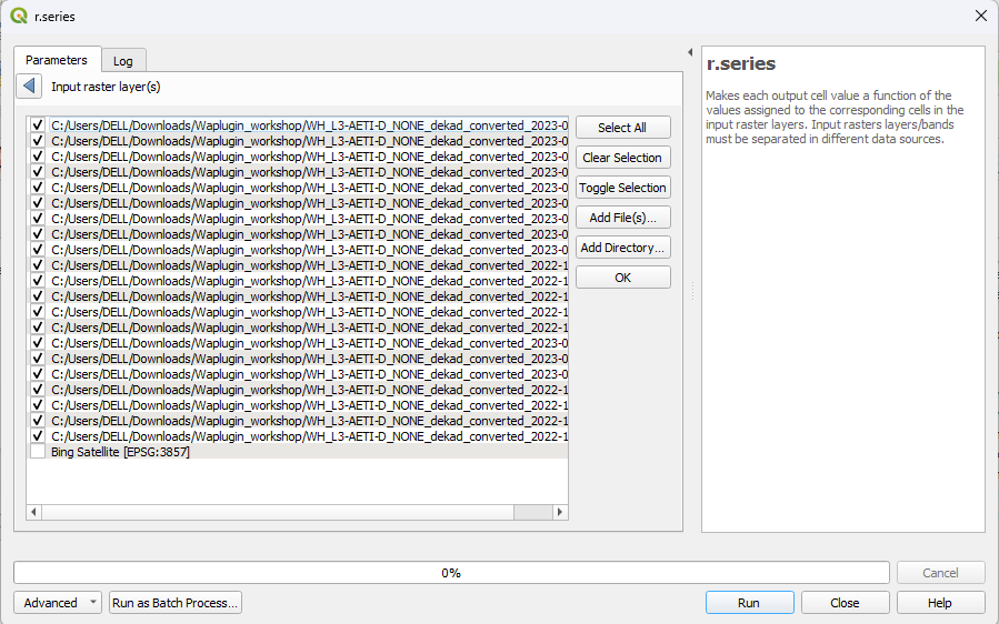
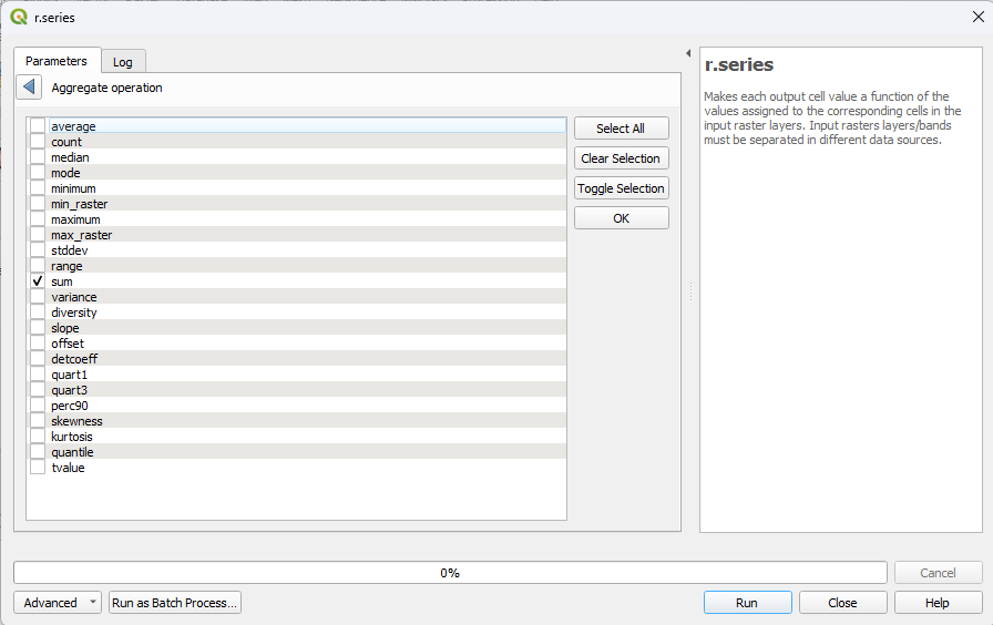
3. Double-click on r.series to open the tool dialog, which allows for the aggregation of multiple rasters.
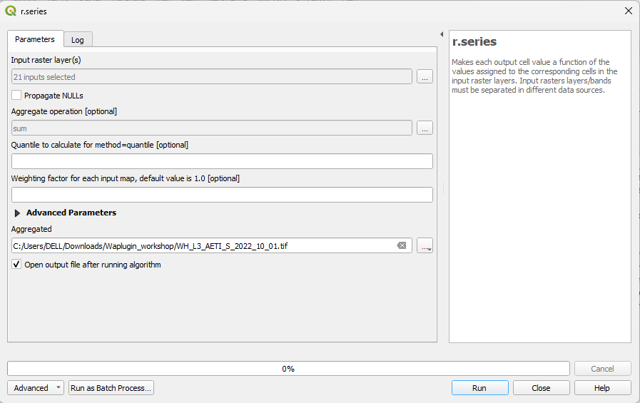
4. At the Input raster layer(s) field, click
 .
.5. Click the Add Files button.
6. Browse to the Waplugin_workshop folder where you stored the downloaded rasters.
7. Select all 21 AETI rasters (one for each dekadal period in the season) and click on Import.
 to go back.
9. In the Aggregate Operation section, the default option is set to average. Uncheck the average option and check the sum option instead.
- This will sum all the dekadal
AETI rasters to create a seasonal map.
11. Click on Run to start the aggregation process.
13. Repeat the same steps for the Transpiration (T) and Net Primary Production (NPP) rasters:
- For Transpiration, select all
the 21 T rasters, aggregate them using the sum option, and
save the output as WH_L3_T_S_2022_10_01.
- For Net Primary Production,
select all the 21 NPP rasters, aggregate them using the sum
option, and save the output as WH_L3_NPP_S_2022_10_01.
Final Output
- After completing these steps, you will have three seasonal maps:
- AETI (Actual Evapotranspiration and Interception)
- T (Transpiration)
- NPP (Net Primary Production)
- These maps will be used in the next chapter for indicator calculation.
5. Compute Indicators Using Indicators Calculator Tab
Now, using the seasonal maps that we computed previously, we will calculate all 8 indicators provided by the WaPLUGIN.
5.1. Uniformity of Water Consumption (Equity)
We'll start with calculating Uniformity of Water Consumption (Equity).
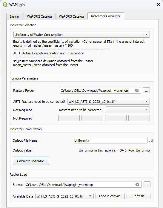
1. Go to the Indicators Calculator tab in the WaPLUGIN.
2. In the Indicator Selection dropdown, select Uniformity of Water Consumption
Consumption Uniformity is measured as the Coefficient of Variation (CV) of seasonal AETI, with the following thresholds:
- CV 0-10% = Good
- CV 10-25% = Fair
- CV > 25% = Poor
3. In the Formula Parameters section, change the path of the rasters folder to the Waplugin_workshop folder.
4. In the dropdown menu, select the seasonal AETI raster (WH_L3_AETI_S_2022_10_01) from the rasters list.
5. Click on Calculate Indicator.
6. The output will be a scalar value displayed in the plugin with the message:
- Uniformity in this region is [value], along with a comment on the uniformity (Good, Fair, Poor).
- Example: For Oued Hellal, the uniformity is 34.5, which is considered poor.
5.2. Beneficial Fraction
The next indicator that we'll calculate is the Beneficial Fraction.
1. In the Indicator Selection dropdown, select Beneficial Fraction.
Beneficial Fraction measures the efficiency of on-farm water and agronomic practices, calculated as the ratio of Transpiration (T) to overall field water consumption (ETa).
2. In the Formula Parameters, select the seasonal Transpiration (T) raster (WH_L3_T_S_2022_10_01) and the seasonal AETI raster (WH_L3_AETI_S_2022_10_01).
3. In the Indicator Computation section, name the output file as WH_BF_2022_10_01.
4. Click on Calculate Indicator.
5. The output is a raster stored in the Waplugin_workshop folder, and it will automatically load into QGIS.
6. Use a nice colour ramp to style the raster.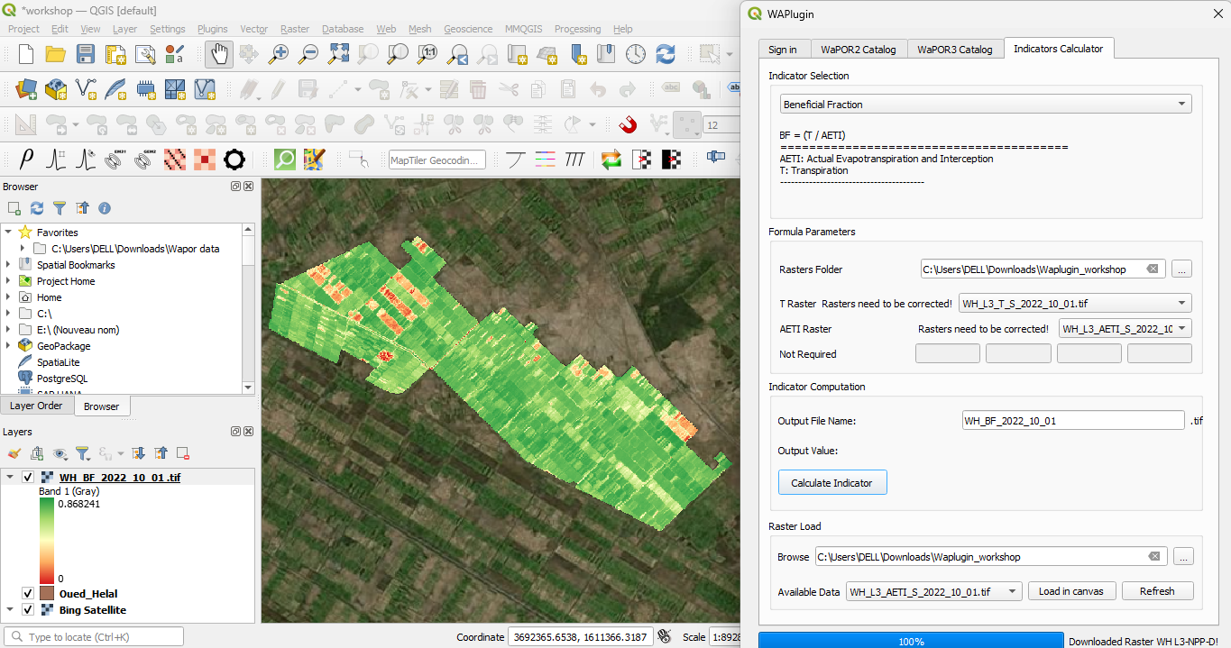
5.3. Adequacy (Relative Evapotranspiration)
Now we're going to calculate the Adequacy indicator.
1. In the Indicator Selection dropdown, select Adequacy (Relative Evapotranspiration).
2. In the Formula Parameters, select the seasonal AETI raster (WH_L3_AETI_S_2022_10_01).
3. Name the output file as WH_Adequacy_2022_10_01.
4. Click Calculate Indicator to compute the adequacy, which will be saved as a raster.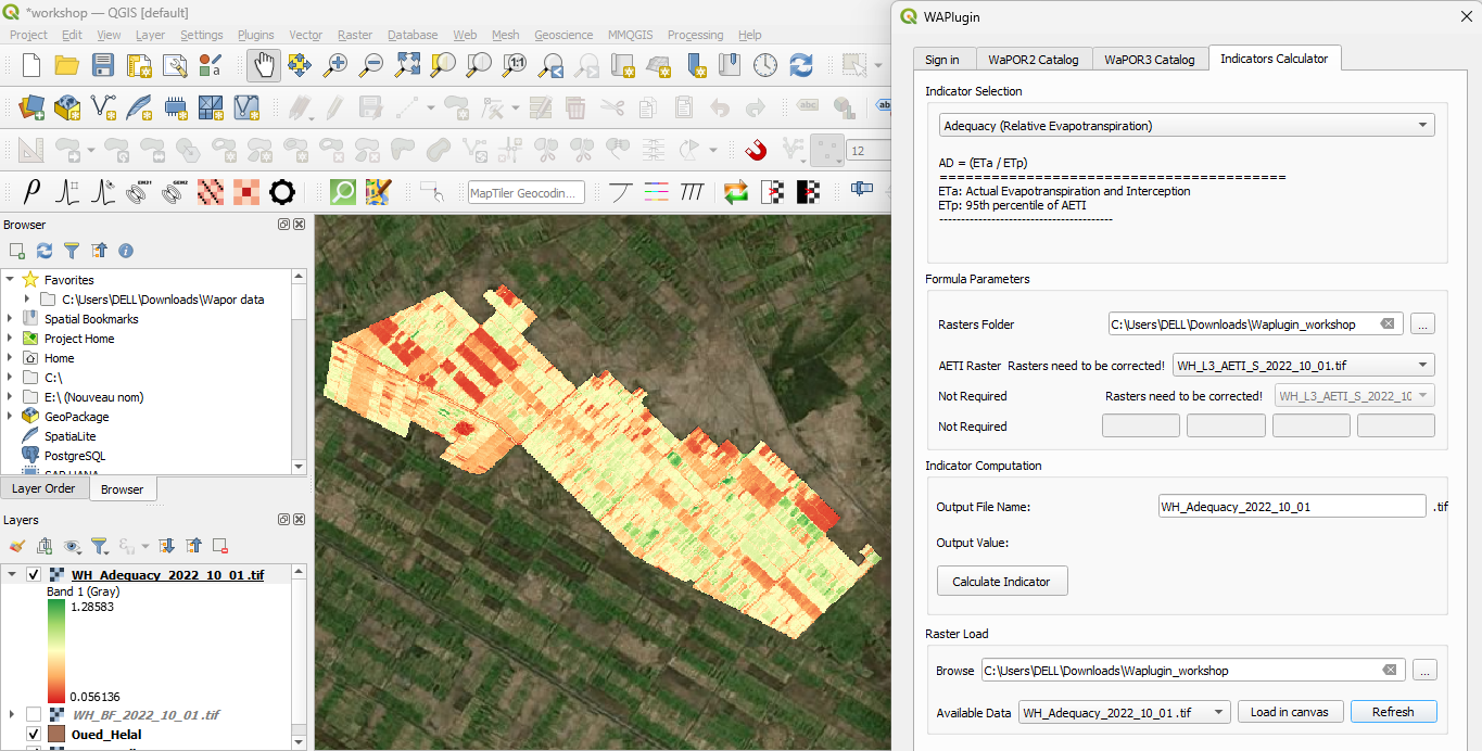
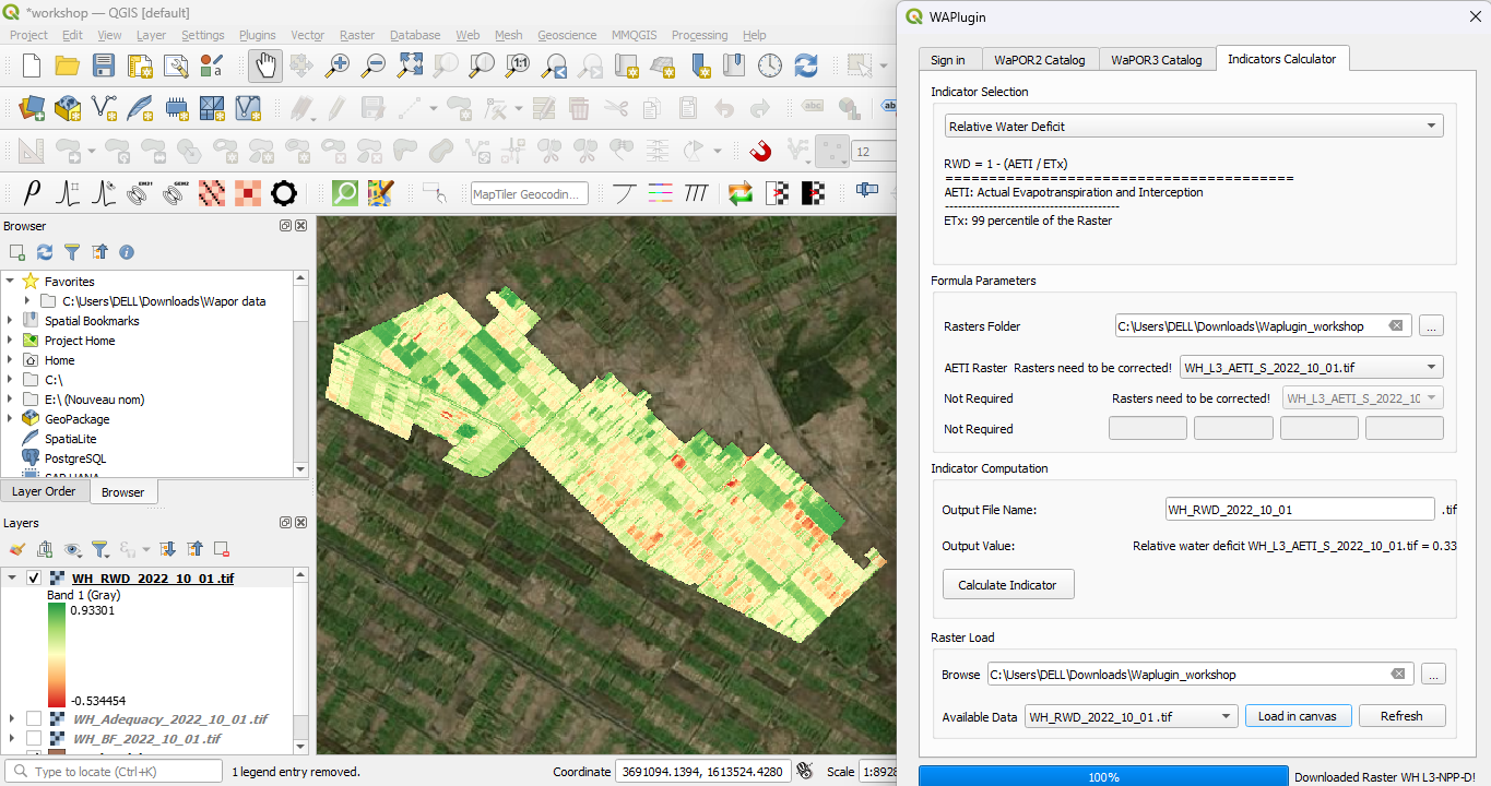
5.4. Relative Water Deficit (RWD)
The next indicator is the Relative Water Deficit.1. In the Indicator Selection dropdown, select Relative Water Deficit.
2. In the Formula Parameters, select the seasonal AETI raster (WH_L3_AETI_S_2022_10_01).
3. Name the output file as WH_RWD_2022_10_01.
4. Click Calculate Indicator. The output will be stored in the Waplugin_workshop folder and displayed as a raster in QGIS.
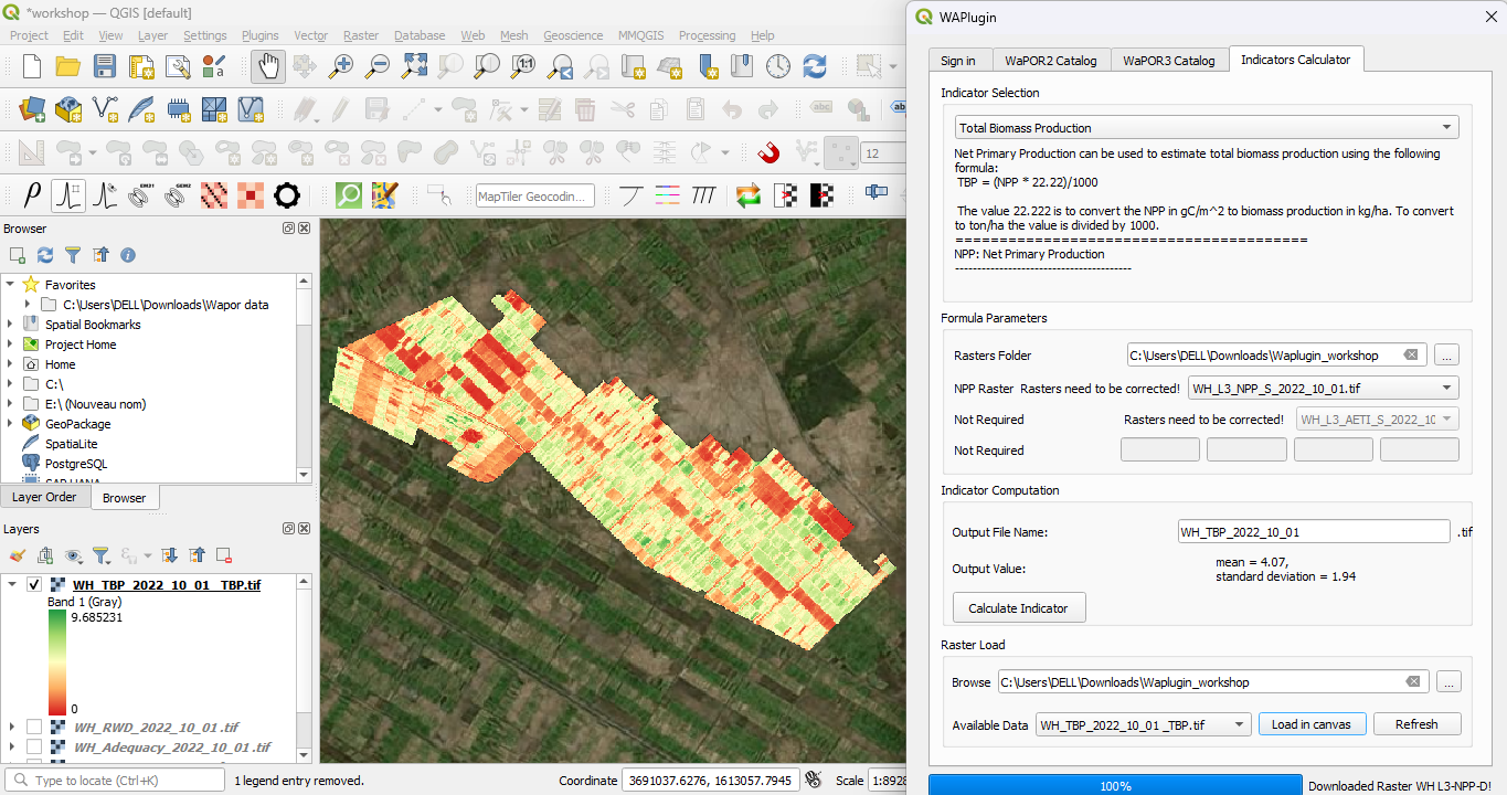
5.5. Total Biomass Production (TBP)
Now we'll calculate the Total Biomass Production.1. In the Indicator Selection dropdown, select Total Biomass Production.
Formula: TBP = (NPP * 22.222) / 1000
This converts Net Primary Production (NPP) from gC/m² to biomass production in ton/ha.
2. In the Formula Parameters, select the seasonal NPP raster (WH_L3_NPP_S_2022_10_01).
3. Name the output file as WH_TBP_2022_10_01.
4. Click Calculate Indicator. The output will be saved in the Waplugin_workshop folder and displayed as a raster.
5.6. Biomass Water Productivity (WPb)
The next indicator is the Biomass Water Productivity.
1. In the Indicator Selection dropdown, select Biomass Water Productivity.
Formula: WPb = (TBP / AETI) * 100. This measures the amount of biomass produced per unit of water consumed.
2. In the Formula Parameters, select the seasonal AETI raster and the Total Biomass Production raster (WH_TBP_2022_10_01) .
3. Name the output file as WH_WPb_2022_10_01.
4. Click Calculate Indicator. The output raster will be saved and loaded into QGIS.
5.7. Yield
We'll calculate now the Yield (kg/ha)
1. In the Indicator Selection dropdown, select Yield.
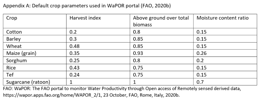
Formula: Y = HI * AOT * fc * (TBP / (1 - MC))
- Parameters for Oued Hellal:
- MC: 0.15 (Moisture content, dry matter over fresh biomass)
- fc: 1.46 (Light use efficiency correction factor)
- AOT: 0.85 (Above ground over total biomass production ratio)
- HI: 0.48 (Harvest Index)
- Note: These parameters are specific to the type of crops that are grown in the study area.
2. In the Formula Parameters, select the Total Biomass Production raster (WH_TBP_2022_10_01).
3. Enter the above parameters and name the output file WH_Yield_2022_10_01.
4. Click Calculate Indicator. The output raster will be saved and loaded into QGIS.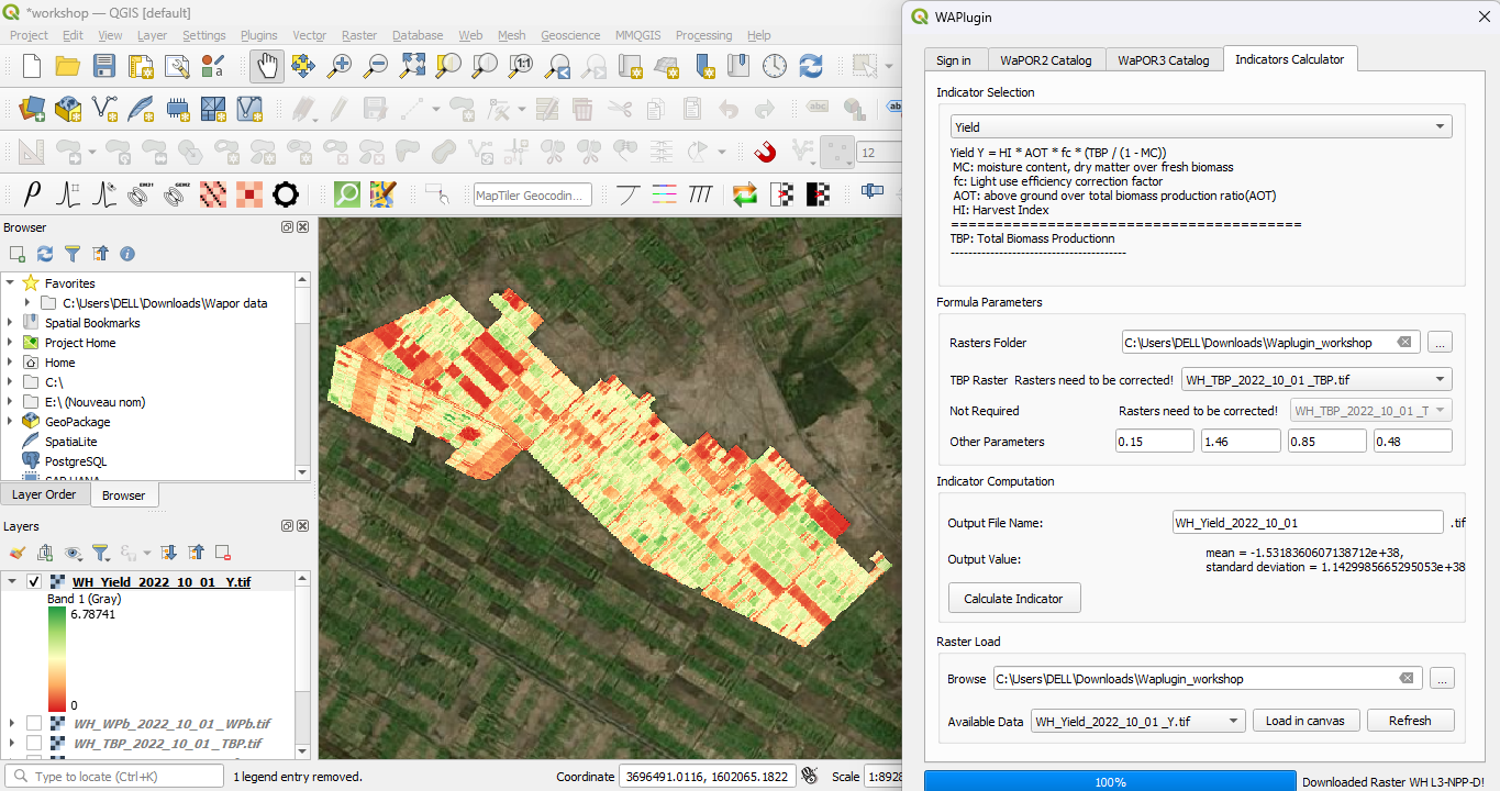
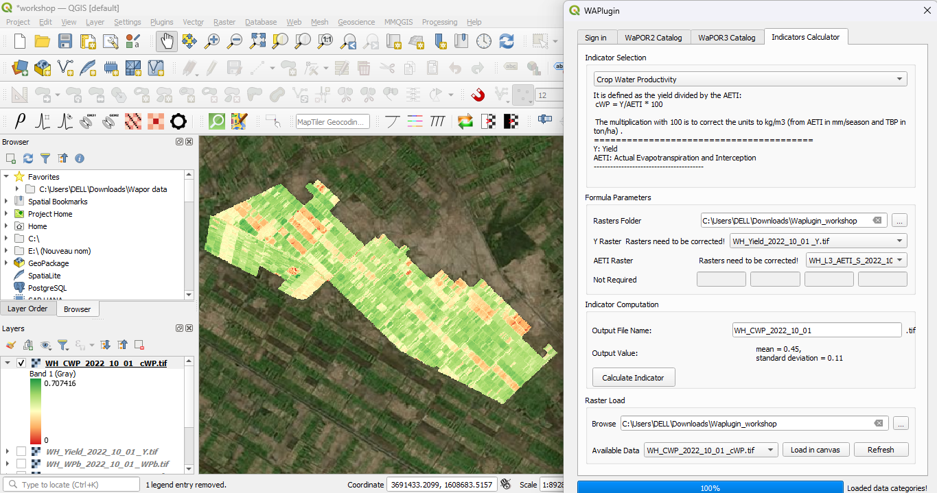
5.8. Crop Water Productivity
Finally, we'll calculate the Crop Water Productivity.1. In the Indicator Selection dropdown, select Crop Water Productivity.
Formula: Crop Water Productivity = Yield / AETI.
2. In the Formula Parameters, select the Yield raster (WH_Yield_2022_10_01) and the seasonal AETI raster.
3. Name the output file as WH_CWP_2022_10_01.
4. Click Calculate Indicator. The output raster will be saved and displayed in QGIS.