Tutorial: Styling Flow Direction with Arrows
| Site: | OpenCourseWare for GIS |
| Course: | Using Mesh Data in QGIS |
| Book: | Tutorial: Styling Flow Direction with Arrows |
| Printed by: | Guest user |
| Date: | Friday, 17 July 2026, 2:32 AM |
Description
1. Introduction
An important layer for hydrologists and water managers is the flow direction. Using colours to style flow direction is possible, but the interpretation is difficult. More intuitive is to style the flow directions with arrows on a background map. This is possible by converting flow direction rasters to mesh format and using the mesh styling panel.In this tutorial, you'll learn to:
- Style a digital elevation model (DEM) with as a colour hillshade using blending.
- Export a flow direction raster to GRIB mesh format.
- Visualise the flow direction mesh with arrows.
Data for this tutorial can be downloaded from the main course page,
2. Styling the DEM
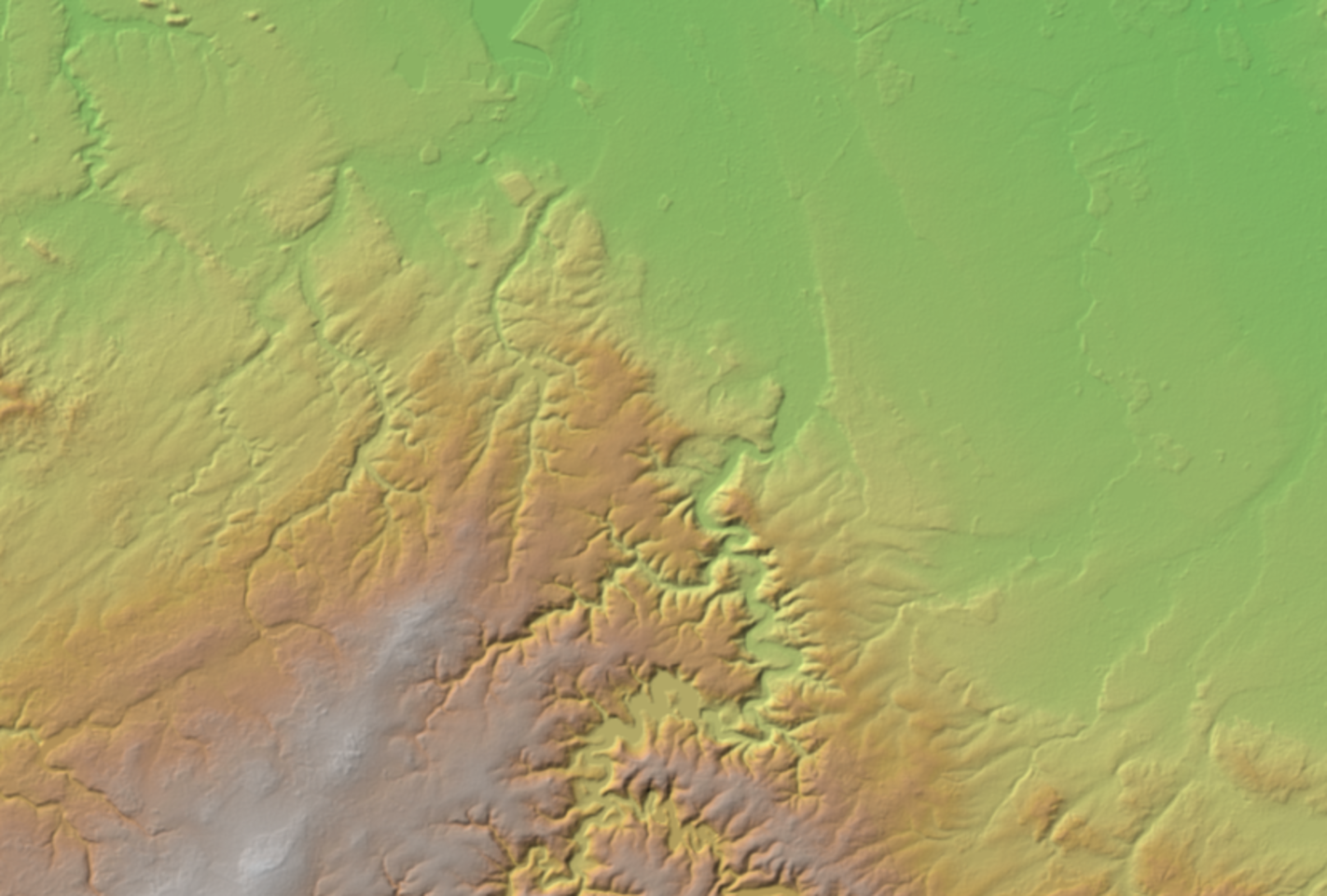
We'll start by preparing a background elevation raster and style it as a colour hillshade.
1. Open QGIS Desktop.
2. Load the provided dem_subset.tif raster in the maps canvas.
By default, QGIS styles raster layers with the Singleband gray renderer. To help interpret the results, it is good practice to intuitively style your layers.
The DEM is a continuous raster. Continuous rasters represent gradients and can therefore contain real numbers ((also called decimal numbers or floating point). Continuous rasters are styled in QGIS using ramps from the Singleband pseudocolor renderer in the Layer Styling panel.
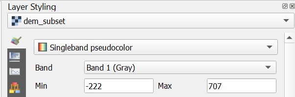
3. Select the dem_subset layer and click ![]() to open the Layer Styling panel (or press
to open the Layer Styling panel (or press F7).
4. In the Layer Styling panel, choose Singleband pseudocolor from the drop-down
list.
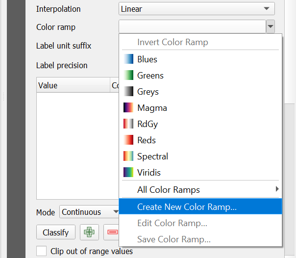
5. Click the arrow at Color ramp and choose
Create New Color Ramp from the dropdown menu.
6. In the popup Color ramp type dialog choose Catalog: cpt-city from the drop-down list.
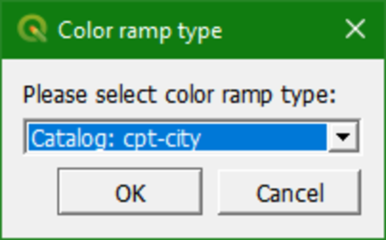
The cpt-city catalog
has a lot of useful preset color ramps.
7. Choose Topography | Elevation. Note that cd-a and sd-a are also nice choices.
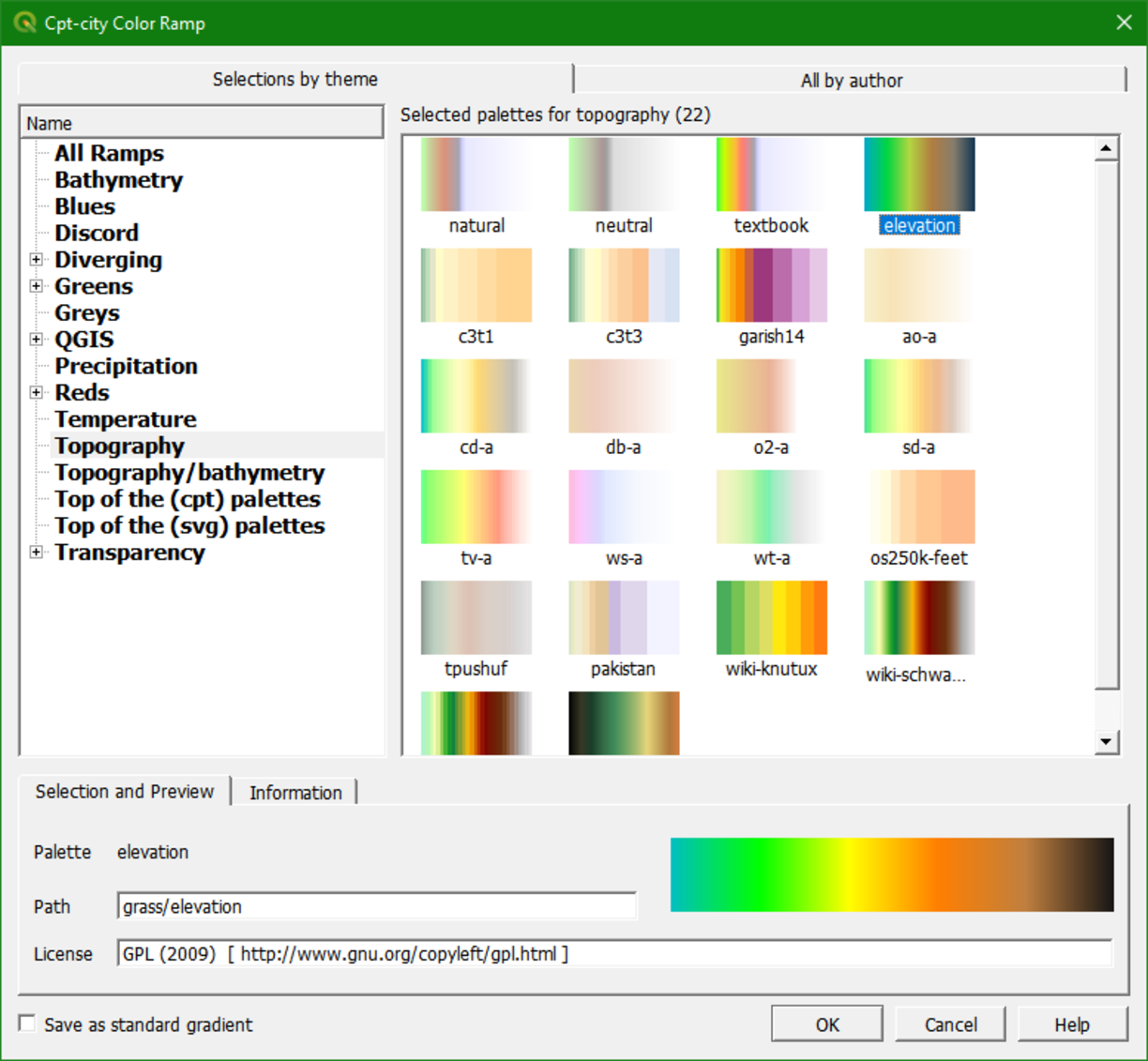
8. Click OK to close the dialog.
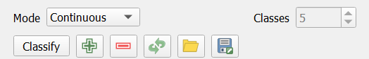
This gives us more intuitive colors in the DEM where we can clearly distinguish higher and lower areas (if you don’t see the colors applied, click Classify).
Now we will further improve the vizualisation.
9. Right-click on the dem_subset layer in the Layers panel and select Duplicate Layer.
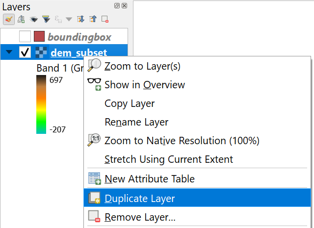
This creates a copy of the dem_subset layer
called dem_subset copy.
10. Uncheck the dem_subset layer, check the dem_subset copy layer and rename it to hillshade.
11. In the Layer Styling panel, which should still be open, make sure that
the hillshade layer is now selected. In the drop-down list change Singleband pseudocolor to Hillshade.
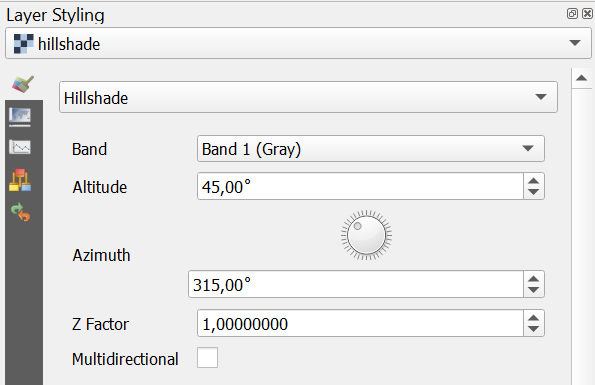
Now the hillshade layer is vizualised with a shading.
- Which direction is the illumination coming from?
- Is this possible in reality?
Hillshade gives the best results with an artificial illumination in the northwest, which in reality can not exist in the Northern Hemisphere. If you move the dial in the Layer Styling panel to the southwest, you will see an inverted relief. Also
note that there is a Resampling section. The default resampling method for both Zoomed in and Zoomed out is Nearest Neighbor. This method is fine for categorical data however, elevation is considered continuous
data. You should therefore choose a Zoomed in resampling method of Bilinear and a Zoomed out resampling method of Cubic.
Next, we're going to blend the DEM with the hillshade layer.
12. Switch
on the dem_subset layer by checking the box.
13. In the Layer Styling panel make sure the dem_subset layer is selected. In the Layer Rendering block of the panel, change the Blending mode to Multiply.
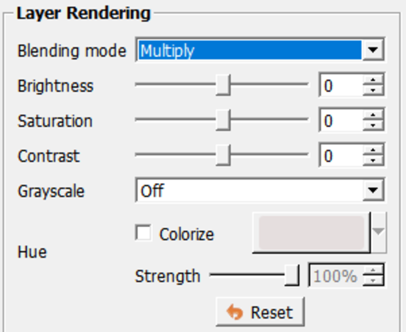
As you can see, blending gives a much nicer
effect than transparency. With transparency the colors will fade. Now we can clearly see the elevation differences: the gradient from south to north and the valleys where we expect the streams.
Blending modes allow for more elegant rendering between GIS layers. They can be much more powerful than simply adjusting layer Opacity. Blending modes allow for effects where the full intensity of an underlying layer is still visible through the layer above. There are 13 blending modes available. See here for more info.
Watch this video to check the steps of this section:
3. Styling the Flow Direction Layer using Arrows
Now add the flowdirection layer and visualize it with arrows on top of the DEM of the previous chapter. This can be done using the mesh styling functionality of QGIS. To use that functionality, we need to convert the flowdirection layer from the PCRaster format to a mesh format. We can do that with the Crayfish plugin.
Instructions to create a flow direction raster from a DEM is covered in another course.
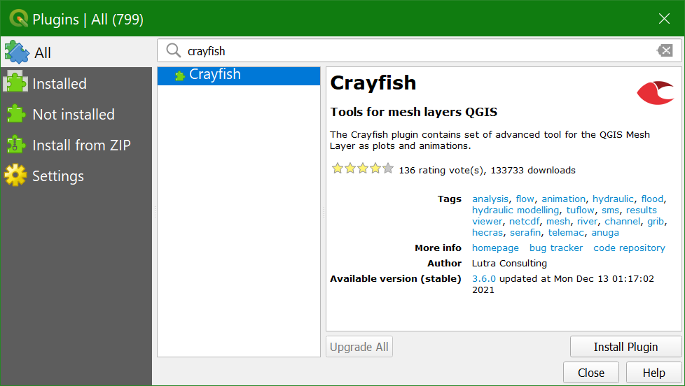
1. Install the Crayfish plugin from the Plugins Manager.
2. In the Processing Toolbox, go to Crayfish | Conversions | PCRaster LDD to GRIB.
Note that flow direction rasters from SAGA are also supported.
3. In the PCRaster LDD to GRIB dialog, choose flowdirection as Input raster and flowdirmesh.grb as Output file (GRIB).
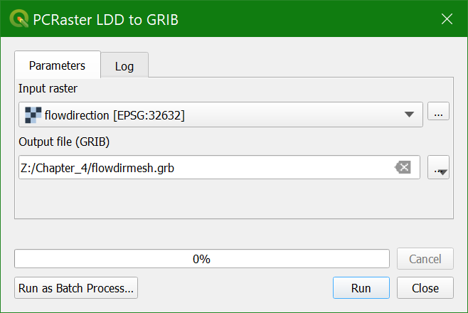
4. Click Run and Close to close the dialog.
5. In the Browser panel, expand the flowdirmesh.grb group (you might need to refresh the Browser panel with the ![]() button) and drag the flowdirmesh layer with the mesh icon
button) and drag the flowdirmesh layer with the mesh icon ![]() to the map canvas.
to the map canvas.
This might take some time. If the file is too large for your computer’s memory, you can get errors. In that case, you can clip the flowdirection layer to a smaller area and repeat the steps to convert the file to the mesh format.
When the map canvas shows a completely yellow layer, the flowdirmesh layer has been loaded and we can start styling it.
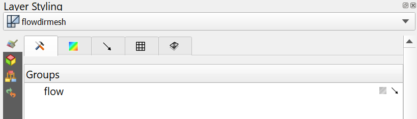
6. Select the flowdirmesh layer in the Layers panel and open the Layer Styling panel.
7. In the Layer Styling panel, go to the Datasets tab and click on ![]() to disable contours and click on the arrow to enable vectors (you might need to enlarge the Layer Styling panel to see these icons).
to disable contours and click on the arrow to enable vectors (you might need to enlarge the Layer Styling panel to see these icons).
Now so many arrows are drawn in the map canvas that it turns black. Let’s tune the settings to improve this.
8. Go to the Vectors tab and change the Arrow Length settings to Fixed and the Length to 2.00. Change the Color to dark blue.
9. Zoom in to see the flow direction with arrows.
10. Check the box to Display on User Grid to show the arrows fixed to a grid, e.g. with an X and Y Spacing of 10 px.
The settings are depending on your zoom level. Play with the settings to get a nice result. You can also try the other Symbology settings for visualization as Streamlines and Traces.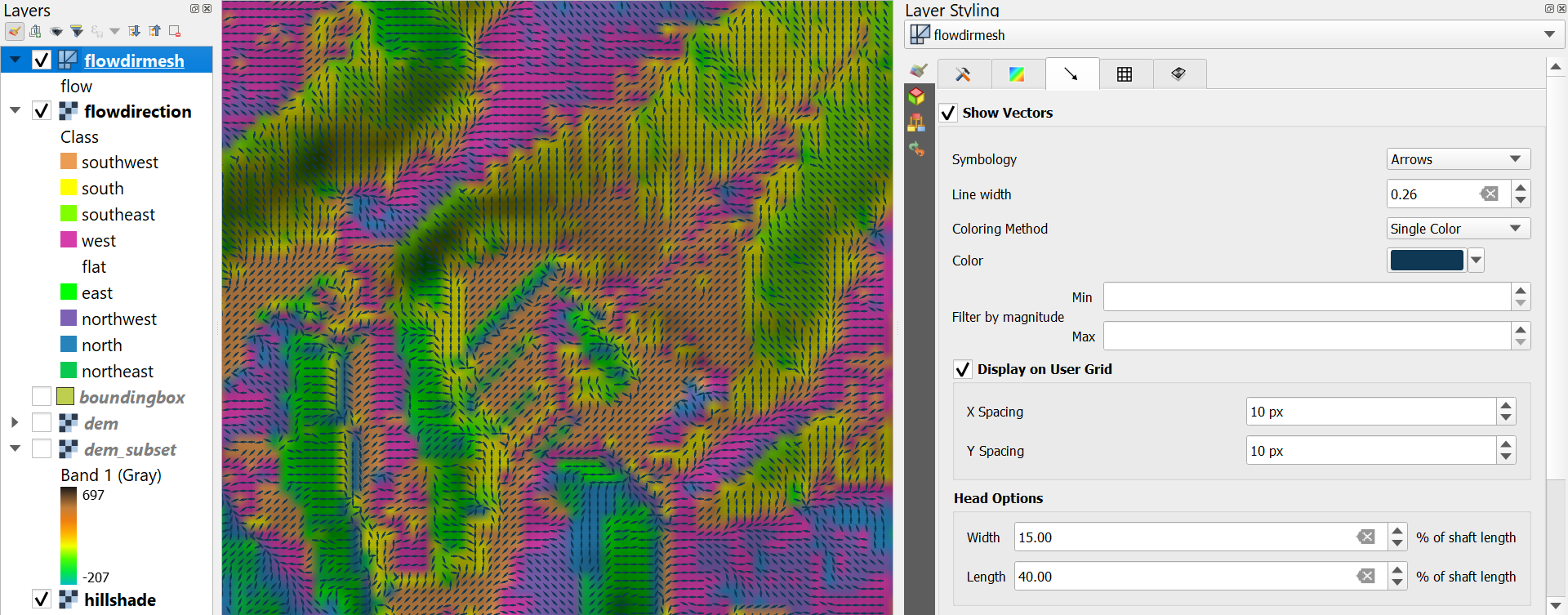
Watch this video to check the steps until this point:
4. Visualize Flow Direction in 3D
We can also visualize the flow direction using the QGIS 3D Map View.
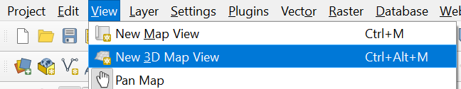
1. In the main menu, choose View | New 3D Map View.
2. In the 3D Map view, click the Options
![]() button and choose Configure....
button and choose Configure....
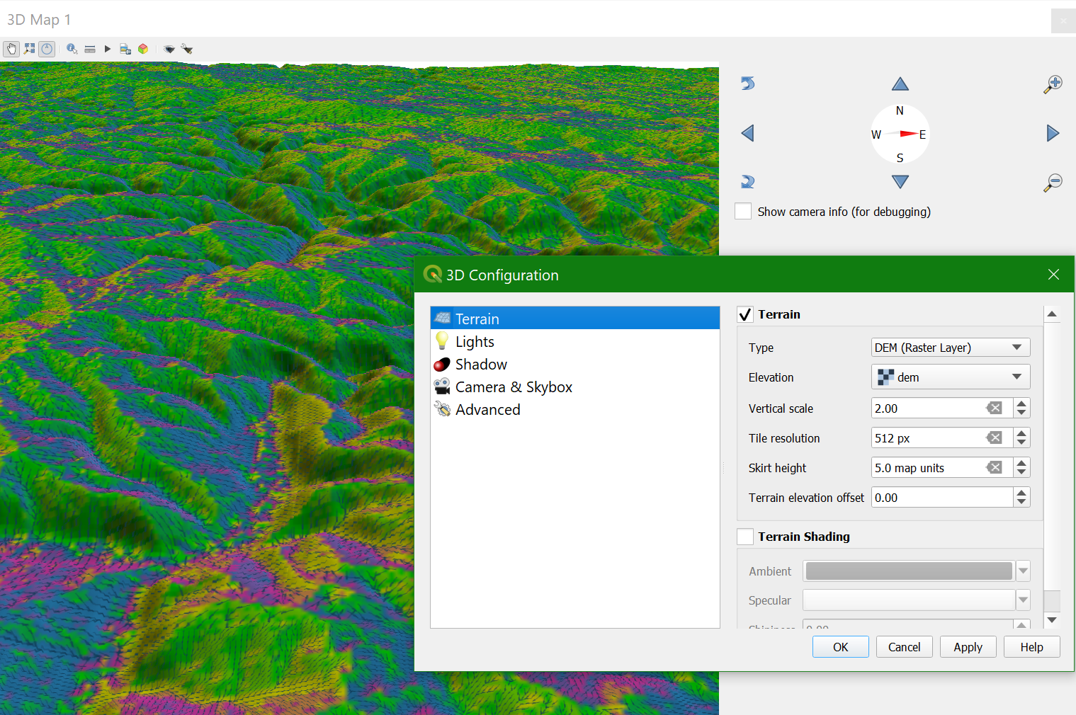
3. In the 3D Configuration dialog, stay in the Terrain tab and change the Type to DEM (Raster Layer) and choose dem as Elevation. Click OK to apply the settings and return to the 3D Map view.
The 3D view will now start rendering. Try to navigate the scene with the different mouse buttons and the compass. You can change the Vertical scale, Tile resolution and Skirt height in the 3D Configuration to improve the visualization.
5. Conclusions
In this lesson you have learned to:
- Style a digital elevation model (DEM) with as a colour hillshade using blending.
- Export a flow direction raster to GRIB mesh format.
- Visualise the flow direction mesh with arrows.