Tutorial: Delineate multiple (sub)catchments
| 站点: | OpenCourseWare for GIS |
| 课程: | Hydrological Analysis in QGIS |
| 图书: | Tutorial: Delineate multiple (sub)catchments |
| 打印: | ゲストユーザ |
| 日期: | 2026年07月27日 星期一 00:27 |
1. Introduction
In this tutorial, we'll delineate multiple (sub)catchments using three methods:
- CSV file with a list of coordinates.
- Using the Pit tool
- Using the junctions of tributaries
2. CSV with outlet coordinates
In the previous tutorial, you have delineated the catchment for one specific outlet. The CSV file that you have created can be extended with multiple locations. Each location should have its own ID number.
1.Open QGIS with the project of the previous tutorial.
2. Define multiple outlet coordinates in a CSV file by repeating this section of the previous tutorial.
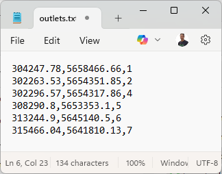
For example, in this screenshot, there are seven outlets for which we want to derive their (sub)catchment. It follows the pattern: x,y,id.
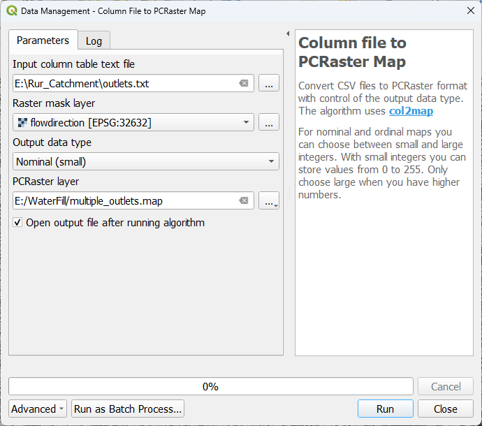
3. With the Column file to PCRaster map we can convert this CSV to a nominal raster with the ID numbers as pixel values.
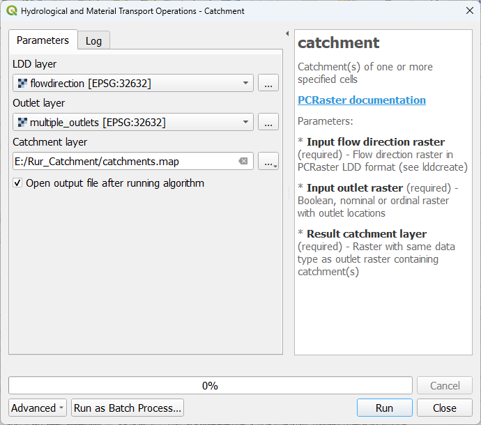
In the previous tutorial, we have used the catchment tool to derive the catchment of the single outlet. Here we can use the same tool for deriving multiple catchments.
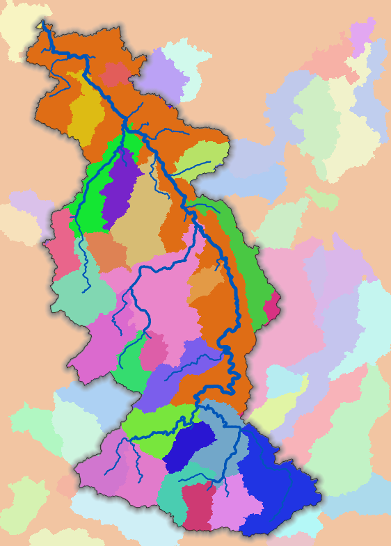
This is then the result. We can apply the same colours as the outlets by copy/pasting the styling.
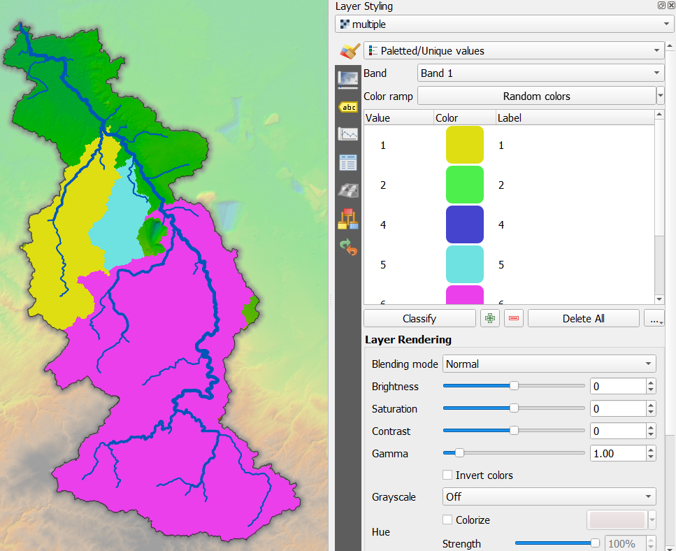
Here you see that you only have three of the seven catchments. If you have defined an outlet upstream of another outlet, the catchment tool will let the downstream catchment absorb the upstream catchment. If you're interested in seeing the division between the two subcatchments, you can use the subcatchment tool.
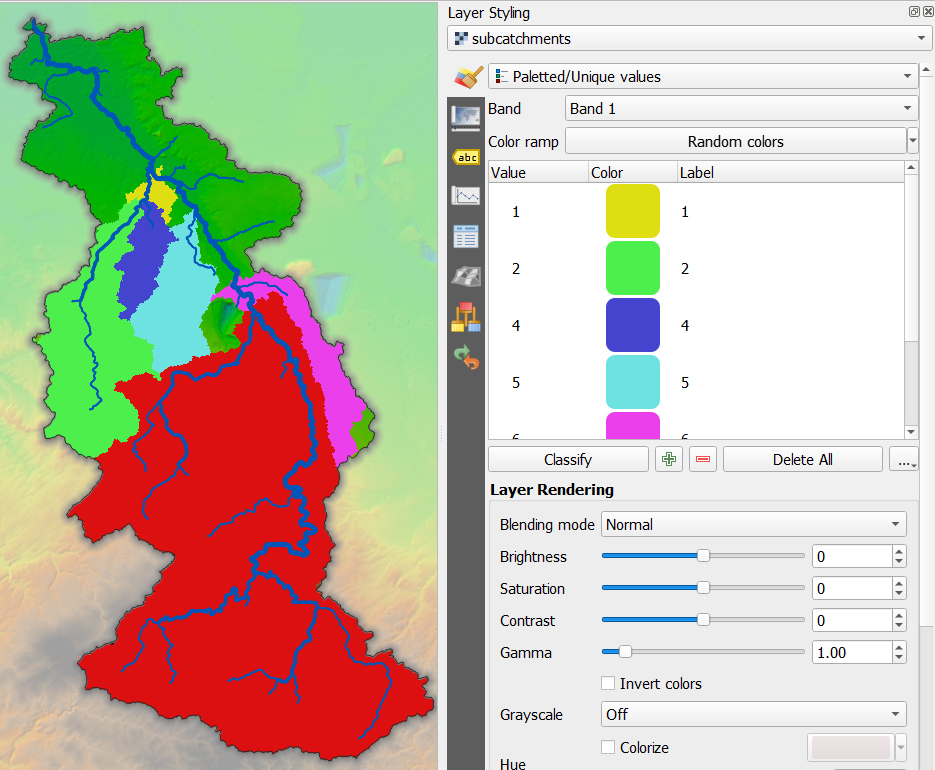
Here you can see the result of the subcatchment tool for the same outlets.
Sometimes you don't have the coordinates and just want the software to determine the outlets automatically. The next chapters show two methods for automatically finding outlets and deriving their (sub)catchments.
3. The Pit Tool
An easy way to find outlets of (sub)catchments in your DEM is to use the pit tool.
A pit is a cell in which all surrounding neighbors have a drainage direction that leads toward the pit cell. Unlike other cells, a pit does not possess a local drainage direction because all adjacent cells are situated at a higher elevation. Additionally, the outflow cell of each catchment—positioned at the edge of the map—is also considered a pit. In a local drainage direction network, pit cells are assigned the value 5.
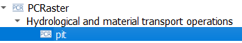
1.In the Processing Toolbox, double click on the pit tool.
2. In the dialog, choose the flowdirection layer as LDD layer and create an Output pit raster layer with the name pits.map.
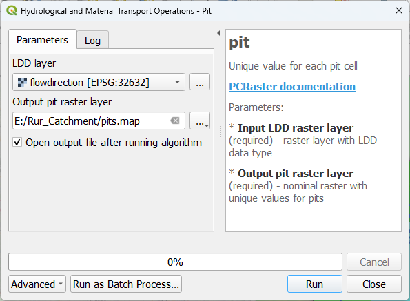
3. Click Run. Click Close after processing.
4. Style the result with Random colors with the Paletted/Unique values renderer in the Layer Styling panel.
You'll see that it has found many pits.
Let's derive their catchments.
5. Use the catchment tool to derive the catchments of the pits layer.
Note that you can more or less recognise the Rur catchment derived in the first tutorial. You can also see a lot of artefacts at the border of the study area.
Here's a video showing an example of using the pit tool:
For automatically deriving all subcatchments, it's more useful to look at the junctions of tributaries. We'll do that in the next chapter.
4. Using junctions
To more precisely derive all subcatchments, we can try to find the junctions where tributaries join. Where tributaries join, the Strahler order downstream is different than upstream. Therefore we can use the Strahler orders in combination with the downstream tool to find the junctions. The downstream tool gets the value of the neighbouring downstream cell. Let's apply this.
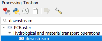
1.In the Processing Toolbox, double click the downstream tool.
2. In the dialog, choose flowdirection as Flow direction layer, channelsstrahler as Raster layer and name the result downstream.map.
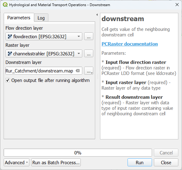
3. Click Run and click Close after processing.
4. In the Layers panel, copy the style from the channelsstrahler layer to the downstream layer.
5. Zoom in on junctions and compare the two layer.
Now we want to have only the cells of the junctions. Therefore we need to use a comparison operator.
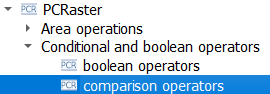
6. In the Processing Toolbox, double click on the comparison operators tool.
7. In the dialog, use channelsstrahler as the first Input raster, != as Comparison operator and downstream as the second Input raster. Save the Output Boolean raster as junctions.map.
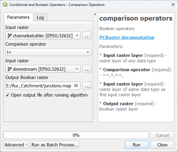
So basically, we've formulated an expression that IF the cell value of the channelsstrahler layer is not equal to the corresponding cell value of the downstream layer, the result raster should have boolean 1 (True), else it should have boolean 0 (False). In that way all junctions will have boolean 1.
8. Click Run and click Close after processing.
9. Style the junctions layer with the Paletted/Unique values renderer and check the result.
Now the problem is that all junctions have the same value. In order to use them in the subcatchment tool, they need to have a unique ID with the nominal data type. Let's fix that.
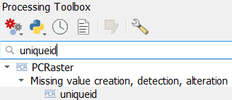
10. In the Processing Toolbox, double click on the uniqueid tool.
11. In the dialog, choose junctions as Input boolean layer and save the Output unique id raster to uniqueid.map.
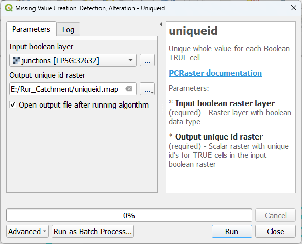
12. Click Run and click Close after processing.
The output is unfortunately in the scalar data type and needs to be converted to the nominal data type before we can use it to derive the subcatchments.
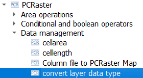
13. In the Processing Toolbox, double click on the convert layer data type tool.
14. In the dialog, choose the uniqueid layer as Input raster layer, Nominal as Output data type and save the Output raster layer as outlet_junctions.map.
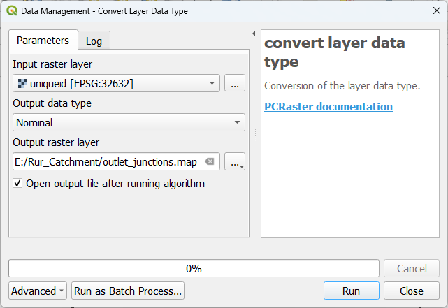
15. Click Run and click Close after processing.
16. Style the result with the Paletted/Unique values renderer and check the result.
It is no problem that the non-junction river pixels have value zero, because the subcatchment tool will only consider non zero cells as outlets.
17. Go to the subcatchment tool and use the outlet_junctions layer as Outlet layer. Save the result as subcatchment_junctions.map.
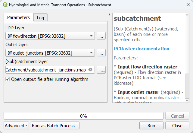
18. Click Run and click Close after processing.
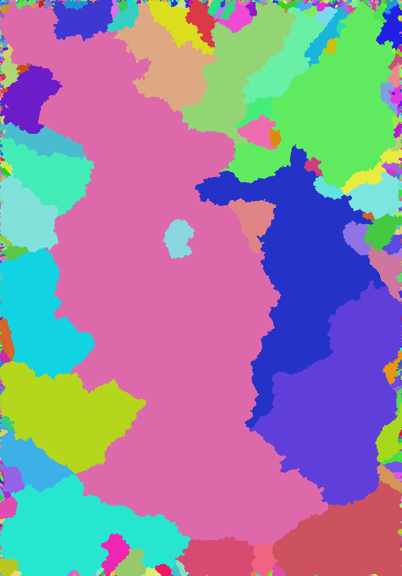
19. Style the result with the Paletted/Unique values renderer.
The result should look like this: