Tutorial: Introduction to GDAL
| Site: | OpenCourseWare for GIS |
| Course: | Programming Basics for QGIS Users |
| Book: | Tutorial: Introduction to GDAL |
| Printed by: | Guest user |
| Date: | Friday, 19 June 2026, 11:33 AM |
Table of contents
1. Introduction
What is GDAL
GDAL is a translator library for raster and vector geospatial data formats that is released under an MIT style Open Source License by the Open Source Geospatial Foundation. As a library, it presents a single raster abstract data model and single vector abstract data model to the calling application for all supported formats. It also comes with a variety of useful command line utilities for data translation and processing.
Starting with GDAL 3.11, parts of the GDAL utilities are available from a new single gdal program that accepts commands and subcommands. In this tutorial, we'll use this new GDAL CLI. See for more info: http://www.gdal.org.
Learning objectives
After this course you will be able to:
- Retrieve information from GIS data
- Reproject GIS data
- Change raster properties
- Convert raster formats
- Convert vector formats
- Apply spatial queries on vectors
- Convert comma separated values files
- Perform batch conversion
Software
For these exercises GDAL needs to be installed, preferably using the OSGeo4W distribution package. If you have installed QGIS, the OSGeo4W distribution is already there. In the video you can see how to install the LTR version of QGIS and Jupyter Lab, which we will also use later in this course.
Note that you need QGIS 3.40.14 or later to use the new GDAL commands.
Exercise data
roads.shp: road map from OpenStreetMap (http://openstreetmap.org)
srtm_37_02.tif: tile of a Digital Elevation Model (DEM) from the Shuttle Radar Topography Mission (SRTM) (http://www2.jpl.nasa.gov/srtm/)
gem_2011_gn1.shp: borders of Dutch communities, freely available from CBS (Statistics Netherlands) and Kadaster (http://www.cbs.nl).
Locations.csv: table with object locations.
landuse.zip: contains land-use time series in IDRISI format.
2. Using the OSGeo4W Shell
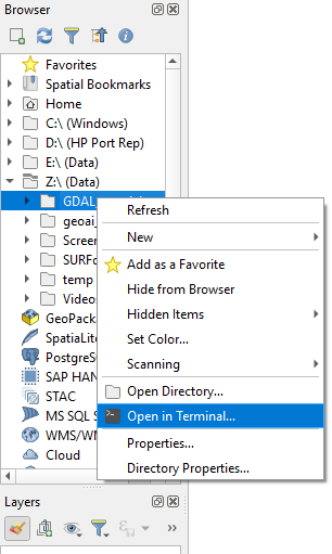
In this tutorial we'll use GDAL shipped with QGIS. You can use the GDAL commands through the OSGeo4W shell. The easiest way of opening the shell is through the QGIS Browser panel.
- Start QGIS Desktop
- In the Browser panel, locate the folder where you have saved the data for this tutorial, e.g. Z:\GDAL_tutorial.
- Right-click on the folder name and choose Open in Terminal... from the context menu.
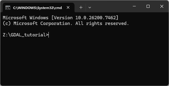
In the OSGeo4W terminal that has opened now you can see at the prompt that you are in the directory of the tutorial data.
Let's first check if your CLI works with the latest gdal commands.
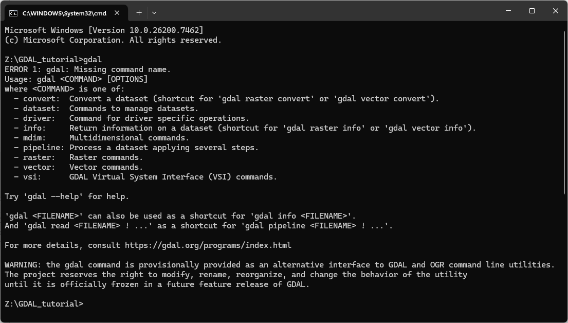
3. Execute the following command:
gdal
If you see this as the result, all is fine:
If the
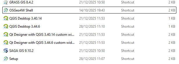
gdalcommand is not recognised, you probably have an outdated version of QGIS with its related OSGeo4W Shell. If you're sure that you're using a newer version, try to locate the shortcut to the OSGeo4W shell in the following way:
- Go to the Start menu.
- Type
QGISto search for QGIS Desktop 3.40 or newer- Click on Open file location
- Run OSGeo4W Shell from here.

You're now set to type gdal commands at the prompt. In the next chapters, you'll learn some of the most used commands.
3. Retrieving information from GIS data
In this chapter you will learn how to:
- Retrieve information from raster data
- Retrieve information from vector data
gdal info command.3.1. Retrieve information from raster data
One of the easiest and most useful commands in GDAL is gdal
info. When given a raster, vector or multidimensional raster dataset as an argument, it retrieves and prints all relevant information that is known about the file. This is especially useful if the GIS data contains additional tag data, as is the case with TIF files. When working with satellite imagery, this is an extremely useful way of keeping track of the images location in long/lat coordinates as well as the image projection. Although the command gdal raster info existis for rasters, gdal info is a shortcut that can detect if your input is raster or vector. Therefore, you don't need to specify raster or vector in the command..
1. Execute the following command:
gdal info srtm_37_02.tif <ENTER>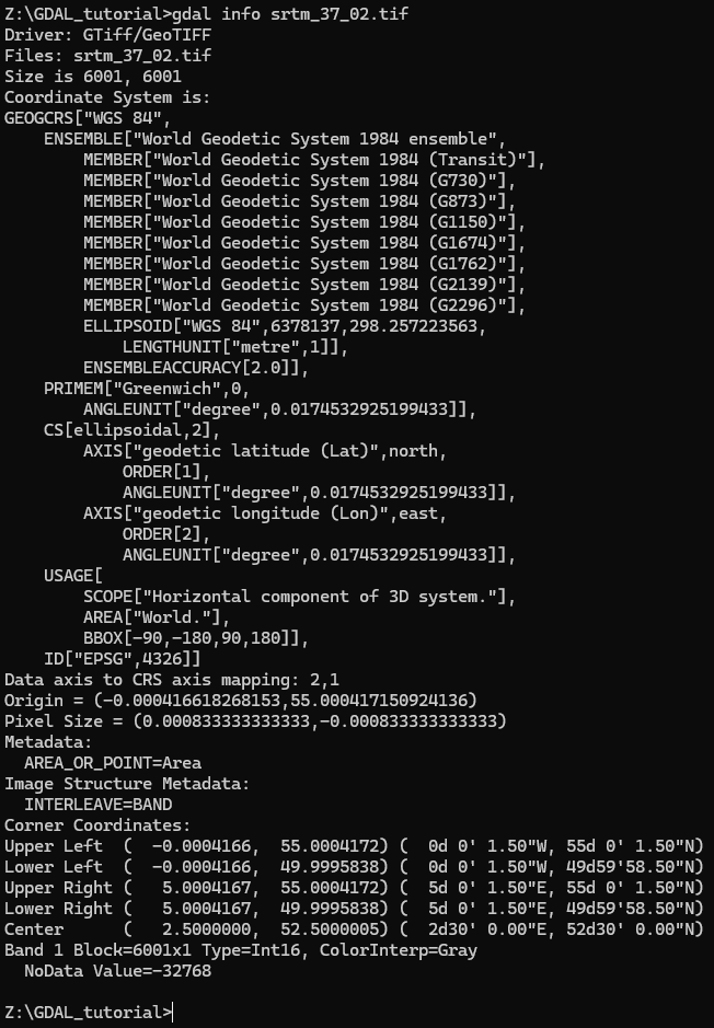
- What is the size of the image?
- What is the coordinate system?
- What is the EPSG code?
- What is the NoData value?
- What is the data type?
gdal
info command can be found at https://gdal.org/en/stable/programs/gdal_info.html#gdal-info3.2. Retrieve information from vector data
For retrieving info from vector data we use the gdal vector info command. However, we can also use the same gdal info command.
1. Execute the following command:gdal info roads.shp <ENTER>gdal info gem_2011_gn1.shp <ENTER>

2. Answer these questions:
- What are the projections of these two shapefile?
- What are the EPSG codes?
roads.shp is EPSG: 4326, which means that it is in Geographic Coordinate System (GCS) with coordinates in Latitude/Longitude.gem_2011_gn1.shp the projection is EPSG: 28992, which is the Dutch projection (Amersfoort RD/New).gdal vector info --features gem_2011_gn1.shpgdal vector info --features --limit 1 gem_2011_gn1.shpThis will show only the first feature, so we have overview of the fields in the attribute table.
More info about the gdal info command can be found here.
4. Reprojecting GIS data
In this chapter you will learn to:
- Reproject raster data
- Reproject vector data
gdal raster reproject and gdal vector reproject commands.4.1. Reproject raster data
GDAL has the capability to reproject a raster file using the following syntax:
gdal raster reproject -d EPSG:... <input> <output>
The -d argument specifies the target coordinate system. If the source coordinate system is unknown it must be specified with the -s argument. EPSG:... specifies the EPSG code of the projection. <input> and <output> are the input and output data respectively.
We are now going to reproject a Digital Elevation Model (DEM) acquired by the Shuttle Radar Topography Mission (SRTM). You can download DEM's for your own area of interest from USGS Earth Explorer. Here we'll use the provided course data.
In order to reproject the DEM from WGS-84 lat/lon to Amersfoort/RD New we use this command:
gdal raster reproject -d EPSG:XXXXX srtm_37_02.tif dem_rd.tif
1. Replace XXXXX with the proper EPSG code for Amersfoort/RD New (see one of your previous answers using gdal info).
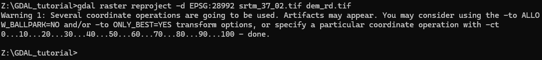
2. Execute the command:
gdal raster reproject -d EPSG:28992 srtm_37_02.tif dem_rd.tif <ENTER>
3. Visualize the result in QGIS.
More info on the gdal raster reproject command can be found here.
Note that by default nearest neighbour resampling is used. Check the command arguments in the documentation if you want to use another resampling method and control the output cell size.
4.2. Reprojecting vector data
For vector data the gdal vector reproject command is used to reproject vector data. The syntax is:
gdal vector reproject -d EPSG:XXXXX <input> <output>
Here we'll convert the OpenStreetMap road data to the Amersfoort/RD New projection.
1. Execute:gdal vector reproject -d EPSG:28992 roads.shp roadsreprojected.shp
The command is executed (it takes some time), but gives a warning.
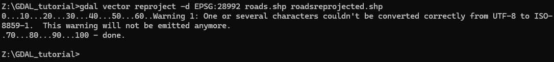
2. What does the warning mean?
More information about the gdal vector reproject command can be found here.
5. Convert GIS formats
In this chapter you'll learn how to
- Convert between different raster formats
- Convert between different vector formats
gdal raster convert and the gdal vector convert commands.5.1. Convert raster formats
The primary function of gdal raster convert is to convert between raster formats. The basic syntax is:
gdal raster convert -f FORMAT <inputFile> <outputFile>
All supported formats can be found here. For FORMAT you should use the Short Name from the table.
Now we are going to convert the DEM from GeoTiff to SAGA format. SAGA is a GIS which has its own -gdal-supported- binary format with the .sdat file extension.
1. Execute the following command:gdal raster convert -f SAGA dem_rd.tif dem_rd.sdat

Some formats need more arguments. PCRaster for example needs a specification of the data type (boolean, nominal, scalar, etc.). Let's convert the same data to PCRaster format.
PCRaster is a software library for environmental modeling and map algebra, widely used in hydrology, ecology, and geography. It provides operators for spatial analysis, dynamic modeling, and simulation of environmental processes. In QGIS, PCRaster is available through the PCRaster Tools plugin, which integrates its functions directly into the Processing Toolbox so users can run PCRaster operations within QGIS.
2. Execute the following command:gdal raster convert -f PCRaster --co VS=SCALAR dem_rd.tif dem_rd.map
This gives the following error:

GDAL is expecting a Float32 raster. When you have checked the information with gdal info, you might have seen that the data type of our DEM is INT16. Therefore, we first need to convert the data type of the input.
3. Execute the following command:
gdal raster set-type --ot Float32 dem_rd.tif dem_rd_float.tif

4. Now you can do the conversion by executing this command:
gdal raster convert -f PCRaster --co VS=SCALAR dem_rd_float.tif dem_rd.map

To convert to PCRaster format you need to know the data type of the raster. In the example above the DEM is continuous data, so the data type is scalar. If the layer was discrete (classes) then the data type was nominal. The table below shows the data types withe the corresponding --ot and --co arguments for respectively gdal raster set-type and gdal raster convert.
| Data Type | --ot |
--co |
|---|---|---|
| Boolean | Byte |
VS=BOOLEAN |
| Nominal | Int32 |
VS=NOMINAL |
| Ordinal | Int32 |
VS=ORDINAL |
| Scalar | Float32 or Float64 |
VS=SCALAR |
| Direction | Float32 or Float64 |
VS=DIRECTION |
| LDD | Int32 |
VS=LDD |
More info about gdal raster convert can be found here.
More info about gdal raster set-type can be found here.
5.2. GDAL raster pipeline
The last example of the previous section would have been more efficient if it could be run at once, without writing the intermediate step of changing the data type. For these purposes, there is the gdal raster pipeline command.
Let's apply it to the entire workflow that does the following steps without writing the intermediate results to disk:
First we need to delete the existing intermediate results to be sure that we create new data.
- Execute the following command to delete all files starting with
dem:del dem*.*
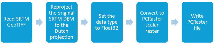
2. Now we can write the pipeline:
gdal raster pipeline read srtm_37_02.tif ! reproject -d EPSG:28992 ! set-type --ot Float32 ! write dem_rd.map -f PCRaster --co VS=SCALAR
Explanation:
- The command to create a raster pipeline is
gdal raster pipeline. - We have to start with reading the input raster:
read srtm_37_02.tif. - Each following processing step needs to be indicated by
!. - First we reproject:
reproject -d EPSG:28992. - Then we set the data type of the result of that step to Float32:
! set-type --ot Float32. - Next we write the result to PCRaster format with scalar data type:
! write dem_rd.map -f PCRaster --co VS=SCALAR.

In conclusion: pipelines are an easy way to create workflows that can be executed in one go. In combination with batch files this can be very easy and powerful without the requirement to write scripts in Python.
5.3. Convert vector formats
gdal vector convert command.gdal vector convert -f FORMAT <inputFile> <outputFile>FORMAT is the Short Name in the vector drivers table.gem_2011_gn1.shp to a Google KML file that can be opened in Google Earth.gdal vector convert -f KML gem_2011_gn1.shp gem.kml gdal vector convert command. Note that you can also use pipelines with vector processing using gdal vector pipeline. More information can be found here.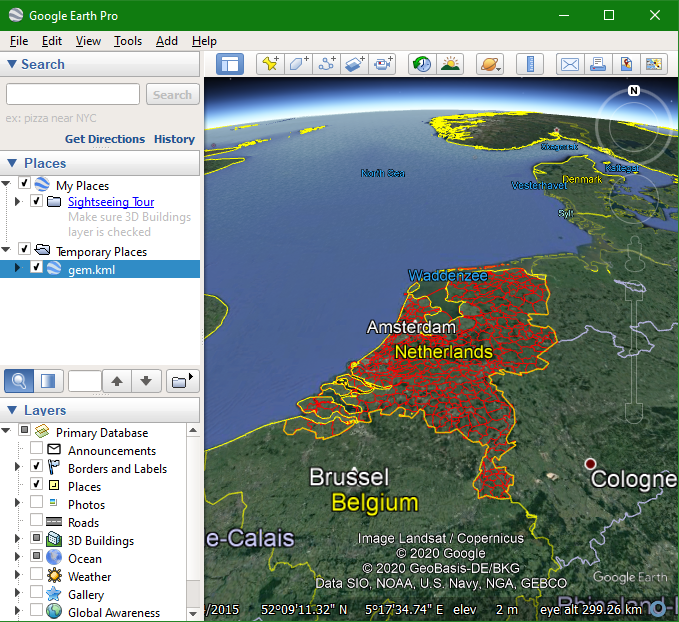
6. Spatial queries of vector data
For our map of Delft we want to do the following GIS analysis:
- Select the municipality of Delft from the municipality map (gem_2011_gn1.shp) and save it into a geopackage;
- Clip the road road map of the Netherlands with the polygon of the municipality of Delft.
gdal vector sql command.
SQL stands for Structured Query Language, and it’s the standard language used to work with relational databases. In GIS, you encounter SQL whenever you filter features, select attributes, join tables, or run spatial queries.
At its core, SQL lets you:
-
Retrieve data (e.g.,
SELECT * FROM municipalities) -
Filter data (e.g.,
WHERE GM_NAAM = 'Delft') -
Update or modify data
-
Create or delete tables
gdal info or QGIS to answer this question.gdal vector sql gem_2011_gn1.shp delft.gpkg --output-layer municipality --sql "SELECT * FROM gem_2011_gn1 WHERE GM_NAAM = 'Delft'"SELECT * FROM gem_2011_gn1 WHERE GM_NAAM = 'Delft' and is asking the database to return all rows from the table gem_2011_gn1 where the column GM_NAAM has the value Delft. Note that Delft is in single quotes to indicate that we're looking for a string (text).roadsreprojected.shp vector so it only covers the municipality of Delft. We use the gdal vector clip.gdal vector clip roadsreprojected.shp delft.gpkg --update --like delft.gpkg --like-layer municipality --output-layer roads_delft
-
gdal vector clip→ the GDAL subcommand to clip vector features. -
roadsreprojected.shp→ the input shapefile containing road geometries. -
delft.gpkg→ the GeoPackage that contains the clipping layer (in this case, the municipality boundary). -
--update→ tells GDAL to update the existing GeoPackage instead of creating a new file. -
--like delft.gpkg --like-layer municipality→ specifies that the clipping should use the layer called municipality insidedelft.gpkgas the mask. -
--output-layer roads_delft→ the name of the new layer that will be written into the GeoPackage, containing only the roads clipped to the Delft municipality boundary.
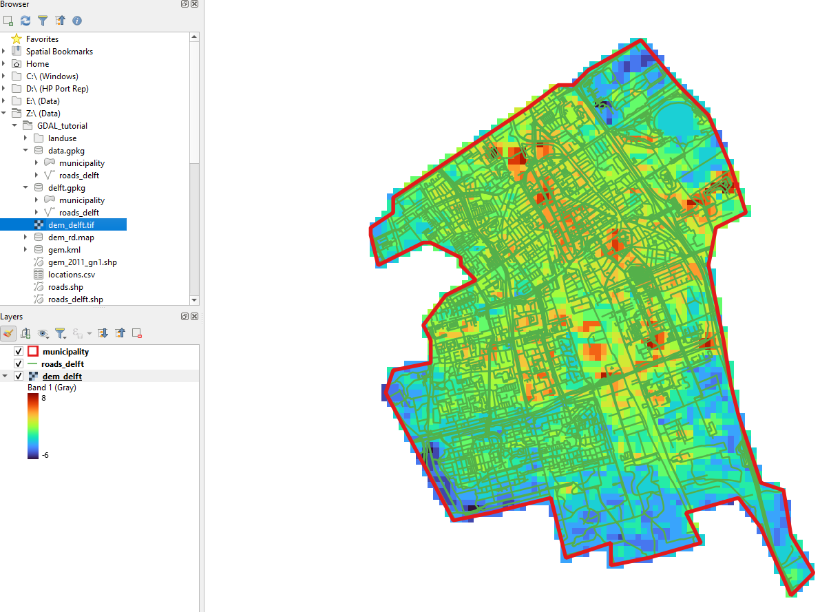
dem_rd.map), the clipped road map (roads_delft) and the community of Delft (municipality).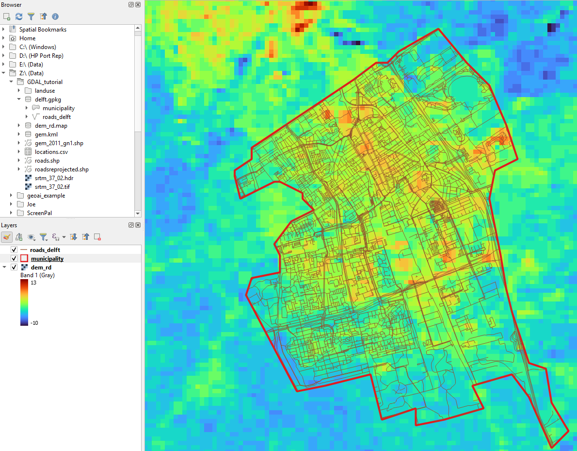
If you check the documentation of gdal vector clip, you'll notice that you could have taken a shortcut. We can add the SQL query to lookup the municipality of Delft to the command.
Let's create the result now as a shapefile so we can compare it with the previous result in the geopackage.
5. Execute the following command:
gdal vector clip roadsreprojected.shp roads_delft.shp --like gem_2011_gn1.shp --like-sql "SELECT * FROM gem_2011_gn1 WHERE GM_NAAM = 'Delft'"6. Add roads_delft.shp to QGIS and compare it with the previous result. It should be the same.
7. GDAL vector pipeline
As with raster data, we can also create pipelines with vector data using the gdal vector pipeline command. Because we can only read input data in the first step and write results in the last step, we're going to create two pipelines. We write the results to a new geopackage called data.gpkg.
Pipeline 1: Extract the Delft municipality polygon
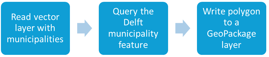
- Execute the following command:
gdal vector pipeline read gem_2011_gn1.shp ! sql --sql "SELECT * FROM gem_2011_gn1 WHERE GM_NAAM = 'Delft'" ! write data.gpkg --output-layer municipality
Pipeline 2: Reproject roads, clip them to Delft, and write to the same GeoPackage
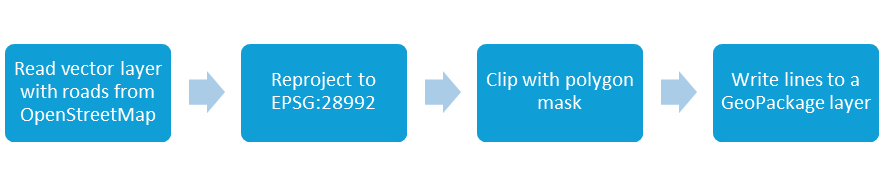
2. Execute the following command:
gdal vector pipeline read roads.shp ! reproject -d EPSG:28992 ! clip --like data.gpkg --like-layer municipality ! write data.gpkg --output-layer roads_delft --update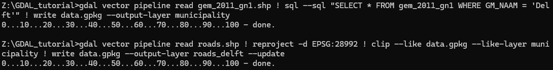
8. Clip raster with a polygon
We can now clip the DEM with the boundary polygon of the municipality of Delft using the gdal raster clip command.
- Execute the following command:
gdal raster clip --like data.gpkg --like-layer municipality -f GTiff dem_rd.map dem_delft.tif - Check the result in QGIS
Assignments
- Check the documentation of
gdal raster clipand try to get the same result by now using SQL to select the municipality from the gem_2011_gn1.shp layer as we did before in other commands. - Create a
gdal raster pipelinefor the workflow that reprojects the srtm_37_02.tif layer to EPSG:28992 and clips it to the municipality of Delft.
9. Convert Comma Separated Values (CSV)
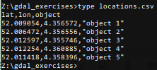
Sometimes you want to reproject coordinates in an ASCII file, e.g. which has been saved to text in a spreadsheet program. Here we will convert the coordinates in a comma separated ASCII file locations.csv to a GeoPaclage point layer with reprojected coordinates.
It is good practice to first view the contents of a CSV file and to verify (1) the coordinates, and (2) the column separator. The separator is not always a comma and sometimes depends on the language settings used while exporting from a spreadsheet programme.
1. View the contents of locations.csv . You can use the type command from the command prompt as you learned in the Command Line tutorial.
<OGRVRTDataSource>
   <OGRVRTLayer name="locations">
      <SrcDataSource>locations.csv</SrcDataSource>
      <GeometryType>wkbPoint</GeometryType>
      <LayerSRS>EPSG:4326</LayerSRS>
      <GeometryField encoding="PointFromColumns" x="lon" y="lat"/>
   </OGRVRTLayer>
</OGRVRTDataSource>
3. Save the file as locations.vrt in the same folder as locations.csv.
Some explanation about the XML file:
<OGRVRTLayer
name="locations">
should correspond with the<SrcDataSource>locations.csv</SrcDataSource><LayerSRS>EPSG:4326</LayerSRS>should correspond with the EPSG code of the coordinate columns
<GeometryField
encoding="PointFromColumns" x="lon" y="lat"/>
indicates the columns with the coordinates that you want to convert.
gdal vector reproject -d EPSG:28992 locations.vrt data.gpkg --update --output-layer locations_reprojectedgdal info. 10. Batch conversion
Desktop GIS applications are great for one‑off operations, but they become inefficient when you need to repeat the same task for many files. In those cases, simple scripting can save a lot of time. You have already explored pipelines. Here we'll create a loop in a batch file.
.rst) format, with one file per year from 1990 to 2030. Our goal is to convert all of them to the GeoTIFF (.tif) format.landuse.zip provided with the course data to a new folder and check the contents.gdal raster convert -f GTiff 01_State19900101.rst 01_State19900101.tif
for %%f in (*.rst) do ( echo Converting %%~nf gdal raster convert -f GTiff "%%f" "%%~nf.tif" )
rst2tif.bat in the folder with the land-use rasters (don't forget to change the extension if you use Notepad, classic mistake!)*.rst files in the folder. %%f is the variable that contains the filename of each file. With echo we can print something to the screen. Here we print %%~nf , which is the part of the filename before the dot that separates it from the extension. Then we use the gdal raster convert command with output format GeoTiff. At the end of the line we add the .tif extension to the filename. The quotes around the file names were added to take care of spaces in file names.rst2tif <ENTER>6. Check the results
11. Conclusion
In this introduction to GDAL, you explored the essential commands for reprojecting, converting, and clipping GIS data. These tools form the foundation for efficient geospatial workflows, enabling you to handle raster and vector formats with confidence. By practicing the examples, you now have a solid starting point for integrating GDAL into your own projects, whether through the command line or within QGIS. With these skills, you can build more advanced pipelines and apply GDAL’s versatility to real-world spatial analysis and mapping challenges.
This video shows the latest updates of GDAL from the developers: