مادة تدريبية: تجهيز بيانات من خرائط ورقية
| الموقع: | OpenCourseWare for GIS |
| المقرر: | تطبيقات في الهيدرولوجيا باستخدام QGIS |
| كتاب: | مادة تدريبية: تجهيز بيانات من خرائط ورقية |
| طبع بواسطة: | Guest user |
| التاريخ: | الجمعة، 26 يونيو 2026، 4:08 PM |
جدول المحتويات
- 1. مقدمة
- 2. المادة النظرية
- 3. إختيار الإسقاط
- 4. استيراد الخريطة الممسوحة ضوئياً إلى أداة المرجع الجغرافي (Georeferencer)
- 5. ضبط معلمات التحويل
- 6. إضافة نقاط التحكم الأرضية (GCPs)
- 7. تقليل الأخطاء وتنفيذ التحويل
- 8. Verify the Georeferenced Map
- 9. Digitizing Vector Layers from a Georeferenced Backdrop
- 10. Styling the Mountains, Rivers, and Lakes
- 11. Conclusions
1. مقدمة
من أجل استخدام الخرائط الورقية في نظام المعلومات الجغرافية (GIS)، يجب إجراء المسح الضوئي لها وإرجاعها جغرافياً. كما أن الإرجاع الجغرافي ضروري أيضاً لبيانات الاستشعار عن بعد الخام، مثل الصور الجوية والمرئيات الفضائية.
للحصول على أفضل النتائج، إختر خريطة ورقية نظيفة لا تحتوي على الكثير من الطيات. استخدم ماسحاً ضوئياً كبيراً بما يكفي لمسح الخريطة بأكملها. يجب أن تكون دقة وضوح الماسح الضوئي عالية بما يكفي (مثل 1200 نقطة في البوصة - dpi) لضمان الحصول على تفاصيل كافية في الخرائط النقطية (raster) الناتجة.
لإجراء الإرجاع الجغرافي، نحتاج إلى ربط مواقع الصورة الممسوحة ضوئياً بـإحداثيات. وهناك طريقتان:
- جمع نقاط التحكم الأرضية (GCPs) في مواقع واضحة تماماً في الصورة، مثل الجسور و التقاطعات.
- إذا كانت الخريطة الورقية تحتوي على شبكة إحداثيات، يمكنك استخدام الشبكة المطبوعة كمرجع. تأكد من معرفة نظام إسقاط هذه الشبكة، والذي عادة ما يكون مدوناً على الخريطة.
- إيجاد نظام الإسقاط ورمز EPSG الخاص بالخريطة.
- تثبيت الإضافات (Plugins).
- إجراء الإرجاع الجغرافي لخريطة ممسوحة ضوئياً باستخدام نقاط التحكم الأرضية (GCPs) من شبكة إحداثيات.
- استخدام أداة التقاط الإحداثيات.
- استخدام الطبقات المتاحة عبر الإنترنت من إضافة QuickMapServices.
- رقمنة النقاط والخطوط والمضلعات وإضافة الخصائص (Attributes).
- استخدام شريط أدوات التلقط (Snapping).
- دمج الميزات (Dissolve).
- تخزين البيانات في حزمة GeoPackage.
- تنسيق (Style) وعنونة (Label) البيانات الاتجاهية (Vectors).
سيعتمد هذا الدرس مسار العمل التالي :
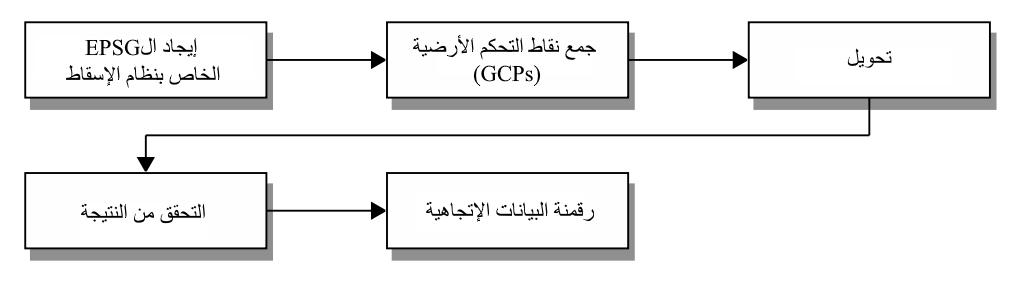
سنستخدم في هذا الدرس خريطة ممسوحة ضوئياً لجبل مارسي (هيئة المسح الجيولوجي الأمريكية - USGS، عام 1979)، والتي تحمل اسم الملف Mount_Marcy_New_York_USGS_topo_map_1979.JPG، حيث سنجري إرجاع جغرافي لها باستخدام شبكة الإحداثيات المطبوعة على الخريطة. يمكن تحميل الملف من صفحة الدرس الرئيسية وحفظه في مجلد محلي، على سبيل المثال: Z:\georeferencing.
2. المادة النظرية
سنقوم بعرض المادة النظرية اللازمة لهذا التمرين في بعض فيديوهات في الأقسام القادمة. يرجى مشاهدة كل فيديو بعناية والإجابة عن الأسئلة الموجودة أسفله. علماً بأن هذه الاختبارات القصيرة ليست تكليفات دراسية، وإنما تهدف لاختبارمعرفتك الشخصية؛ لذا يمكنك المحاولة قدر ما تشاء والتعلم من أخطائك.
2.1. نموذج البيانات الإتجاهية لنظم المعلومات الجغرافية
شاهد هذا الفيديو حول نموذج البيانات الإتجاهية (Vector Data Model) في نظم المعلومات الجغرافية (GIS) ثم أجب عن الأسئلة أدناه.
2.2. إسقاطات الخرائط في نظم المعلومات الجغرافية
شاهد هذا الفيديو حول إسقاطات الخرائط في نظم المعلومات الجغرافية (GIS) وأجب عن الأسئلة أدناه.
2.3. تنسيقات نظم المعلوملت الجغرافية و ممارسات العمل السليمة
شاهد هذا الفيديو حول تنسيقات الGIS و ممارسات العمل السليمة ثم أجب عن الأسئلة أدناه.
3. إختيار الإسقاط
إطلع على الخريطة الممسوحة ضوئياً وحاول معرفة نظام الإسقاط المستخدم في شبكة الخريطة، يمكن إستخدام أي متصفح صور لهذا الغرض.
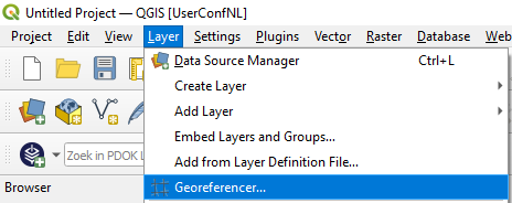
4. استيراد الخريطة الممسوحة ضوئياً إلى أداة المرجع الجغرافي (Georeferencer)
5. ضبط معلمات التحويل
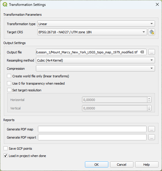
أولاً، علينا ضبط إعدادات التحويل.
- 1. من قائمة أداة الإرجاع الجغرافي اختر Settings | Transformation Settings؛ حيث يمكنك اختيار ما يلي:
- أنواع تحويل مختلفة: يمكن استخدام التحويل الخطي البسيط إذا لم تكن الخريطة مشوهة كثيراً. ويمكن تجربة الأنواع الأخرى عند وجود تشوهات أكبر. تتوفر المزيد من المعلومات حول أنواع التحويل في توثيق برنامج QGIS. سنبدأ بالتحويل الخطي.
- طريقة إعادة أخذ العينات (Resampling method): إذا كنت بحاجة إلى قيم البكسل (pixel values) في حسابات لاحقة، يستحسن إختيار خيار "أقرب مجاور" (nearest neighbor). تحافظ هذه الطريقة قدر الإمكان على قيم البكسل الأصلية باختيار أقرب بكسل. ومع ذلك، تؤدي هذه الطريقة بصرياً إلى خريطة ذات مظهر "مربعات". إذا كان الغرض للاستخدام البصري فقط، كخلفية لترقيم الطبقات الاتجاهية مثلاً، فمن الأفضل اختيار طريقة أخرى. سنستخدم هنا الطريقة "التكعيبية" (cubic)، التي تعتمد على متوسط قيم أقرب 16 بكسل.
- نظام المرجع الإحداثي المستهدف (Target SRS): اختر هنا الكود الذي دونته سابقاً؛ EPSG:26718. يمكنك اختياره بالنقر على زر تعيين الإسقاط
 وكتابة 26718 في حقل التصفية (filter).
2. انتقل إلى المجلد الذي تريد حفظ الخريطة المرجعة جغرافياً فيه باستخدام هذا الزر ![]() تقوم الأداة تلقائياً بإضافة _modified إلى اسم الملف؛ لذا في حالتنا سيكون اسم الملف المرجع جغرافياً Mount_Marcy_New_York_USGS_topo_map_1979_modified.tif. أبقِ الإعدادات الأخرى على وضعها، وقم بتفعيل خيار Load in project when done.
تقوم الأداة تلقائياً بإضافة _modified إلى اسم الملف؛ لذا في حالتنا سيكون اسم الملف المرجع جغرافياً Mount_Marcy_New_York_USGS_topo_map_1979_modified.tif. أبقِ الإعدادات الأخرى على وضعها، وقم بتفعيل خيار Load in project when done.
.
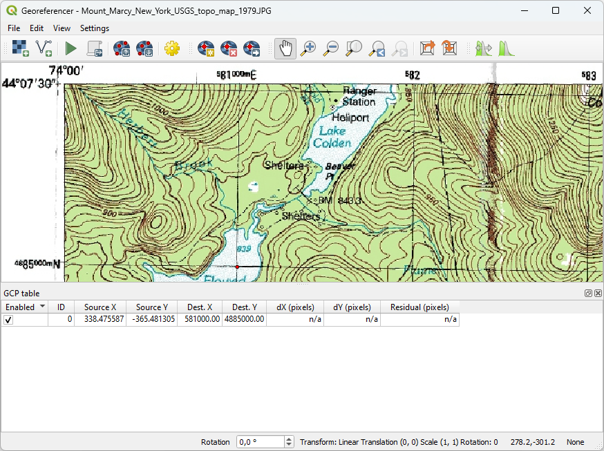
6. إضافة نقاط التحكم الأرضية (GCPs)
من أجل ربط إحداثيات الملف بإحداثيات العالم الحقيقي، نحتاج إلى تحديد نقاط التحكم الأرضية (GCPs) ذات إحداثيات معلومة. يمكننا استخلاص هذه الإحداثيات بطرق مختلفة:
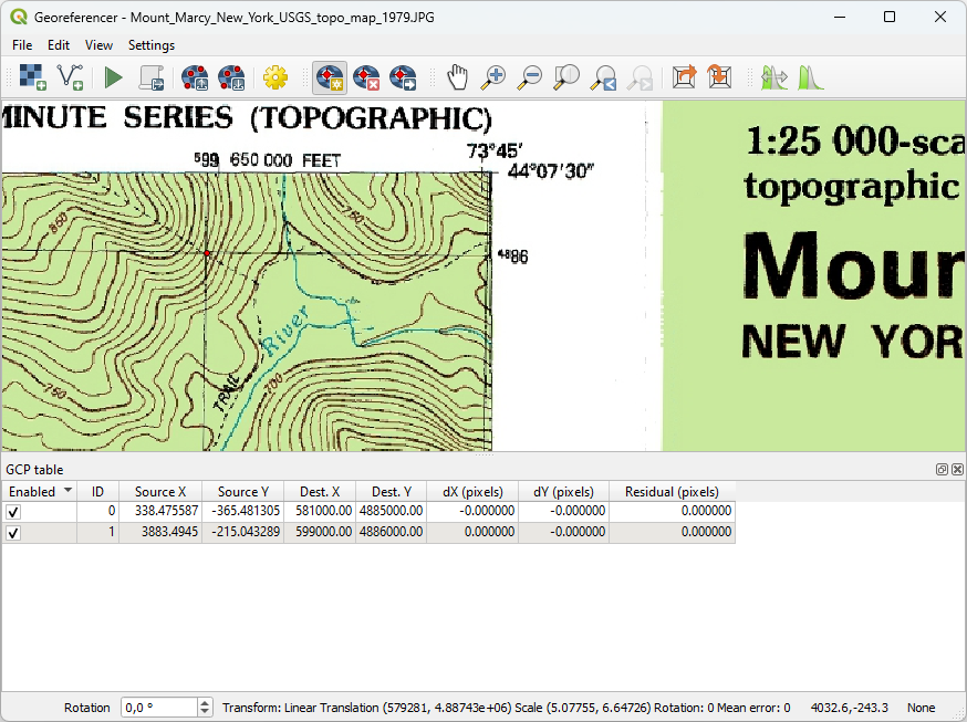
- الطريقة الأسهل هي استخدام شبكة الإحداثيات (coordinate grid) الموجودة على الخريطة الممسوحة ضوئياً، إذا كانت متوفرة وضمن إسقاط معروف. نقوم بالنقر على عقدة (node) في الشبكة ونكتب إحداثيات X و Y المقابلة في مربع الحوار.
- استخدام خريطة مرجعية في نافذة خريطة QGIS تكون مرجعة جغرافياً بالفعل؛ وبهذه الطريقة يمكننا الحصول على الإحداثيات الصحيحة بالنقر على الخريطة المرجعية.
- استخدام نقاط تحكم أرضية تم قياسها في الميدان باستخدام جهاز GPS.
 لإضافة نقطة تحكم أرضية.
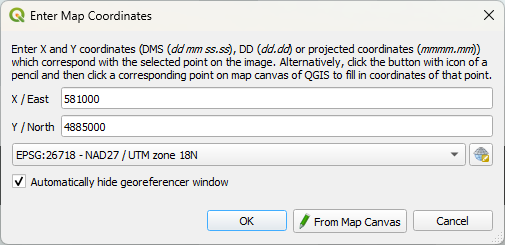
إذا ارتكبت خطأً، يمكنك إزالة نقطة التحكم باستخدام هذا الزر
 .
.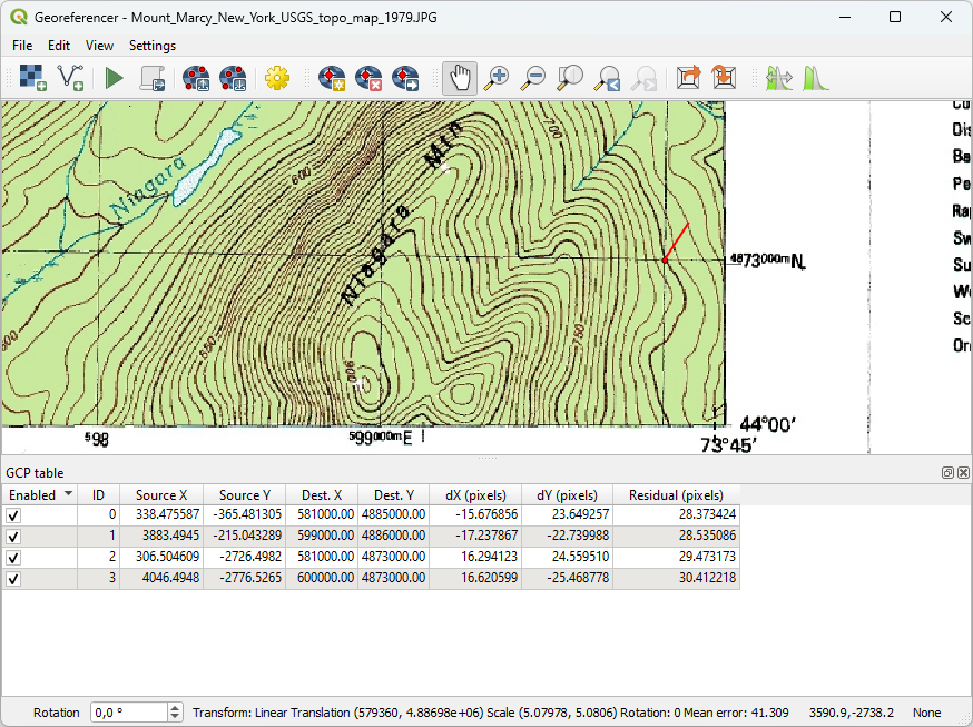
7. تقليل الأخطاء وتنفيذ التحويل
في أسفل الشاشة، يمكنك رؤية خطأ المتوسط التقديري (41.2999 بكسل في حالتنا. يتم تمثيل الخطأ أيضًا بصريًا عند نقاط التحكم الأرضية (GCPs) باستخدام خط أحمر. قيمك لن تكون متطابقة تمامًا و هذا أمر عادي و متوقع.
هناك طريقتان لتقليل الخطأ:
- يمكنك استخدام الزر وضع نقاط التحكم الأرضية
 فعليًا عند العقد المتواجدة قي مناطق تقاطع خطوط الشبكة. ستحتاج إلى التكبير لاختيار الـبكسل الصحيح. لاحظ أن خطأ المتوسط لا يتم تحديثه تلقائيًا؛ بل ستحتاج إلى تغيير نوع التحويل إلى نوع آخر ثم إعادته مرة أخرى.
 - إذا لم يقلل الخيار الأول الخطأ، فيمكننا تغيير نوع التحويل في إعدادات التحويل و بعد هذا سيتم إعادة حساب قيم الخطأ.
في هذا التمرين، سنطبق الخيار الثاني بعد التأكد من وضع نقاط التحكم الأرضية بشكل صحيح.
-
في القائمة، انتقل مرة أخرى إلى الإعدادات | إعدادات التحويل أو انقر أيقونة الترس
 .
. -
الآن لنحدد متعدد حدود من الدرجة الأولى (Polynomial 1) بدلاً من التحويل الخطي. اترك الباقي كما هو.
-
انقر على "موافق" (OK) للعودة إلى جدول نقاط التحكم الأرضية.
الآن يمكنك رؤية أن خطأ المتوسط قد انخفض إلى جزء من البكسل، و هذا مقبول. إذا لم ترَ خطأ متوسط أقل من 1 بكسل، فسيتعين عليك التحقق من مواقع نقاط التحكم الأرضية وتصحيحها.
إعلم أنه لا يمكن دائمًا تحقيق خطأ متوسط أقل من 1 بكسل؛ حيث يعتمد قرار قبول دقة معينة على الخريطة و استعمالاتها.
-
الآن يمكننا بدء الإرجاع الجغرافي باستخدام الزر المخصص
 . تظهر الخريطة المرجعية جغرافيًا الآن في لوحة خريطة QGIS.
 -
يمكنك إغلاق نافذة الإرجاع الجغرافي (Georeferencing). سيسألك البرنامج عما إذا كنت تريد حفظ نقاط التحكم الأرضية (GCPs) الخاصة بك. يمكنك النقر فوق "تجاهل" (Discard) إذا كنت لا تريد استخدامها. إذا قمت بحفظها، يمكنك تحميلها مرة أخرى في إضافة Georeferencing GDAL.
يمكنك تجاهل رسالة التحذير "تم استخدام تحويل تقريبي من EPSG:4326 إلى EPSG:26718".
- انقر علامة (X) لإزالة الرسالة.
شاهد هذا الفيديو للتحقق من الخطوات التي اتبعتها إلى الان :
https://www.youtube.com/watch?v=bKfm0crsMBM
8. Verify the Georeferenced Map
You can verify the result by checking the coordinates at the grid nodes that you used as GCPs.
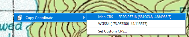
The Map CRS shows the coordinates in the projection of the project (i.e. EPSG:26718), the second field shows the coordinates in the Geographic Coordinate System (i.e. EPSG:4326), with coordinates in decimal degrees of longitude and latitude.
2. Read the coordinates from the side of the map and verify if they correspond with these coordinates. Repeat for the GCP nodes.
Another way to verify the result is to use a web map as a backdrop. The QuickMapServices plugin provides easy access to many web maps such as Google Satellite and OpenStreetMap.
Plugins are third-party additions to QGIS. They can be installed through the Plugins manager. You need an internet connection to connect to the Plugins repository.
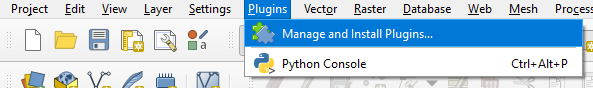
3. Choose from the main menu: Plugins | Manage and Install Plugins...
4. Search for QuickMapServices.
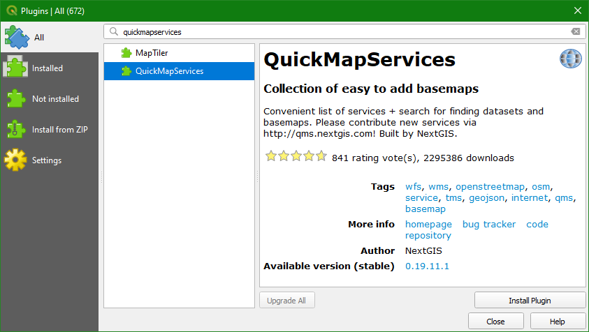
5. Click Install Plugin. Click Close after installing.
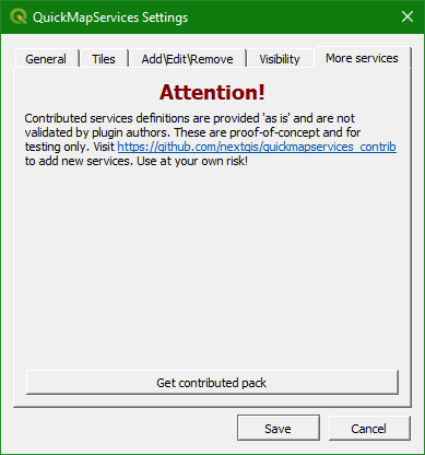
6. In oder to get access to more online resources choose Web | QuickMapServices plugin | Settings from the main menu. Next, choose the More services tab and click Get contributed pack. Click OK in the popup and Save in the dialogue when the contributed pack is installed.
7. Go to the main menu and choose Web | QuickMapServices plugin and select Google | Google Terrain and then OSM | OSM Standard. Compare the georeferenced map with Google Terrain and OpenStreetMap.
To help with this comparison you will employ a Blending Mode. Blending modes determine how two layers interact visually. When a blending mode is applied to a layer it will be blended with the layer below.
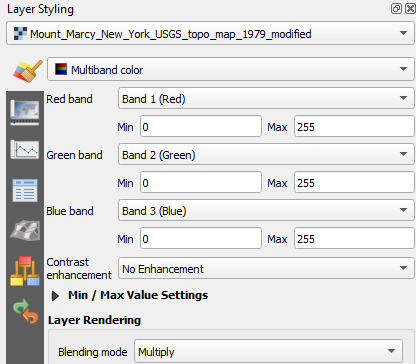
8. Open the Layer Styling panel by clicking the ![]() button. Set the target layer to
button. Set the target layer to Mount_Marcy_New_York_USGS_topo_map_1979_modified.
9. In the panel, choose Blending mode Multiply.
Blending modes allow for more elegant rendering between GIS layers. They can be much more powerful than simply adjusting layer opacity. Blending modes allow for effects where the full intensity of an underlying layer is still visible through the layer
above. There are thirteen blending modes available. A nice overview can be found in this blog by Helen McKenzie.
10. After comparing the georeferenced map with the online layers, change the blending of Mount_Marcy_New_York_USGS_topo_map_1979_modified back to normal. We are going to use this layer in the next sections as a backdrop to digitize vectors. You
can uncheck the Google Terrain and OSM Standard layers.
This is a good time to save your QGIS project (.qgz file).
11. From the main menu, choose Project | Save as... and save it as Exercise_1.qgz in the same folder where you have stored the data.
The project file contains references to all layers (not the data itself), styles, projections, extent and zoom level of the map canvas. Save your project regularly!
Watch this video to check the steps in this chapter:
9. Digitizing Vector Layers from a Georeferenced Backdrop
Our georeferenced scanned map can now be used as a backdrop to digitize vector layers. Vectors can be points, (poly)lines or polygons. In this exercise we are going to digitize:
- Mountain tops as points
- Rivers as polylines
- Lakes as polygons
9.1. Digitize Peaks
First we have to create an empty GeoPackage layer.1. From the main menu select Layer | Create Layer | New GeoPackage Layer.
2. In the New GeoPackage Layer dialogue, first select the Database filename by clicking the ![]() button. Browse to the folder where you want to store the GeoPackage and save it to
button. Browse to the folder where you want to store the GeoPackage and save it to Mount_Marcy.gpkg. For Table name choose Peaks. For Geometry type choose Point. Make sure EPSG:26718
is chosen as the projection. Create a new field with the Name Elevation, Type Whole Number (integer) and click![]() .
.
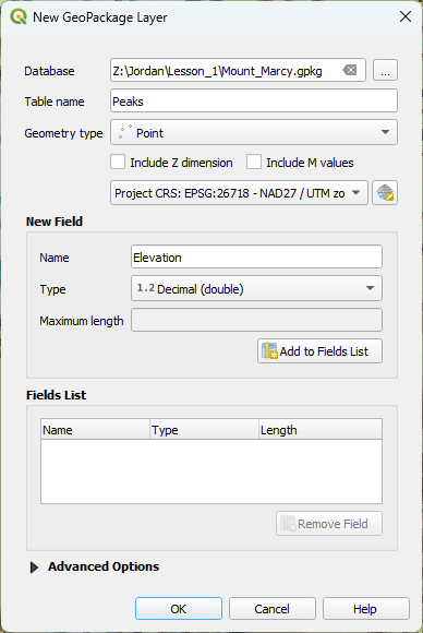
3. Add a second new field with a Type Text named Name. Make sure to click the Add to Fields List button. Then click OK.
The empty layer has now been added to your layers list:
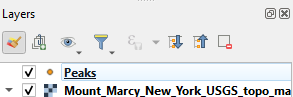
In order to start digitizing, you have to toggle editing mode on.
4. Click on the Peaks layer so it is selected. Click on![]() in the toolbar to toggle to editing mode. You can also right-click on the layer and choose Toggle Editing from the context menu to place the layer into edit mode.
in the toolbar to toggle to editing mode. You can also right-click on the layer and choose Toggle Editing from the context menu to place the layer into edit mode.
Now the buttons on the Digitizing Toolbar become active. A pencil icon also appears next the layer in the Layers Panel indicating the layer is in edit mode.
5. On the topographical map navigate to a mountain. If a geodetic datum is present on top there will be an X and an elevation value.
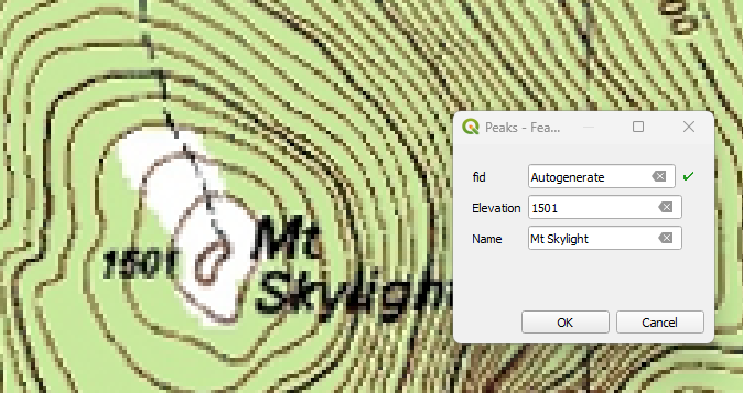
6. When you have found one, zoom in and click the Add Point Feature button ![]() . The cursor changes in a crosshair. Move the mouse to the mountain top. Click on the mountain top.
. The cursor changes in a crosshair. Move the mouse to the mountain top. Click on the mountain top.
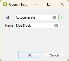
A dialogue with a form shows up. fid is the feature id that is automatically generated. It’s a unique integer number for each feature. The other attributes that we have to fill in are Elevation and Name.
7. In this example we type 1501 and Mt Skylight for Elevation and Name respectively. If you map a peak without a labeled elevation, determine the elevation based on the contour lines.
8. Repeat this step for a few other peaks.
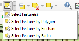
If you made a mistake, you can use the Vertex Tool ![]() to move
the feature or use one of the select options to select the point feature (see screenshot below) and click
to move
the feature or use one of the select options to select the point feature (see screenshot below) and click  to delete the selected point feature. These buttons
 ![]() can be used to undo/redo editing actions. Use
can be used to undo/redo editing actions. Use
![]() to save the edits.
to save the edits.
9. When done, click again on the ![]() button to toggle editing off. If you didn’t save edits yet, it
will ask you to Save or Discard. With Discard you can always undo your edits until the last time it was saved.
button to toggle editing off. If you didn’t save edits yet, it
will ask you to Save or Discard. With Discard you can always undo your edits until the last time it was saved.
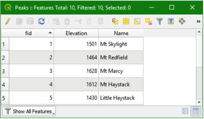
10. You can check the attribute table of your new point vector layer by right-clicking on the layer name (Peaks) and selecting Open Attribute Table.
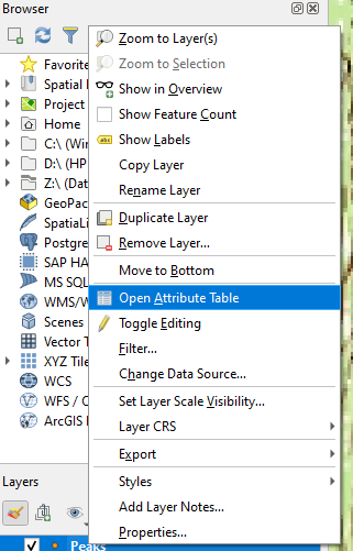
Now you can see the attributes that you have added and their fid, Elevation and Name values:
Watch this video to check the steps of this chapter:
9.2. Digitize Rivers
Your next task is to digitize line features (rivers). The procedure is similar to creating a point layer.
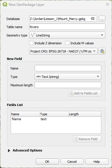
1. In the New GeoPackage Layer dialogue first browse to the existing Database, Mount_Marcy.gpkg.
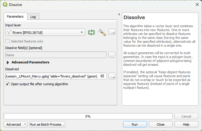
2. Give a new Table name of Rivers and a Geometry type of LineString. Change the projection to the one of the project. As a new attribute we add Name with the type Text data. Don't forget to click the ![]() . Check if the dialogue resembles the figure below and click OK.
. Check if the dialogue resembles the figure below and click OK.
A New GeoPackage Layer window will open informing you that the file already exists.
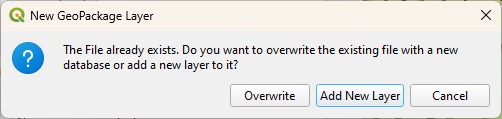
3. Choose Add New Layer.
The Rivers layer is now added to the Layers panel.
4. Toggle editing to start adding rivers. Click on the Add Line Feature![]() button to add a new river feature. Zoom and pan on the map to find a stream to digitize.
button to add a new river feature. Zoom and pan on the map to find a stream to digitize.
Always start digitizing from the upstream to downstream. The direction will be stored in the layer. Always place a vertex when a tributary joins a larger stream. That's important when connecting the tributary later.
5. Click on the starting point of the line (node) and click when necessary to make a vertex.
You can use the zoom and pan buttons to trace the stream. You can use the Spacebar to pan during digitizing. With Backspace you can delete the last node while digitizing.
6. After you place the end node of the line, right click to complete the feature. Now you can enter the attribute data in the form.
Now you are going to digitize a tributary. First you have to set the snapping options.
7. In the main menu choose View | Toolbars | Snapping Toolbar (alternatively right-click on a toolbar and choose Snapping Toolbar). Click ![]() to enable snapping. Choose to snap to vertices of the active layer with a tolerance of 15 meters.
to enable snapping. Choose to snap to vertices of the active layer with a tolerance of 15 meters.
![]()
8. Now digitize the tributary from upstream to where it joins the higher order river. You will see that the line will snap to the node that you placed before on the main river.
If you want all tributaries to be one single feature, you need to dissolve the features.
9. When you have given all tributaries the same name, you can dissolve them by choosing Vector | Geoprocessing Tools | Dissolve from the menu. Use the ![]() button to choose
button to choose Name as the Dissolve field and save the result in a GeoPackage layer with the name Rivers_dissolved.
Click Run.
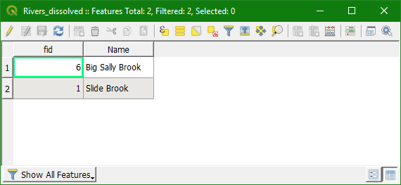
10. Check the attribute table of the result before and after dissolving: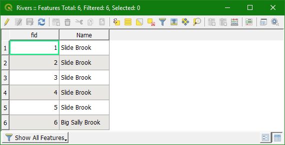
Watch this video to check the steps in this section:
9.3. Digitize Lakes
Finally we are going to create a polygon vector layer for some lakes. Try to find out how to do this for yourself. It is very similar to the procedure for lines. The only difference is that the first node should be the same as the last node in order to close the polygon. Use the name of the lake as a text attribute.
Some lakes have islands that need to be removed from the lake features. For this purpose, enable the Advanced Digitizing Toolbar in a similar way as we enabled the Snapping Toolbar earlier. Click the Add ring button![]() and digitize the island in the same way as you digitize a polygon. After finalizing the ring, it will be removed from the lake polygon.
and digitize the island in the same way as you digitize a polygon. After finalizing the ring, it will be removed from the lake polygon.
The order of the layers is also important. The order of visualization in the map canvas follows the order in the Layers panel. The first layer is on top. The general order of layers is: points, lines, polygons, rasters. Vectors below rasters are not visible, unless you use blending or opacity. This however changes the colors and should only be used if it has a purpose. You can deviate from the general order if that makes the visualization clearer. You can change the order of layers by dragging the layers in the Layers panel to the desired position.
Watch this video to check how to digitize polygons:
10. Styling the Mountains, Rivers, and Lakes
In this final section you will style your peaks, rivers and lakes.
10.1. Style Peaks
You will begin with the styling Peaks layer.
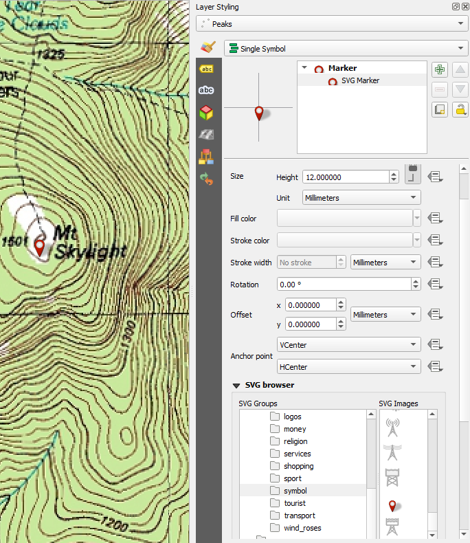
1. Open the Layer Styling panel by clicking the ![]() button. Set the target layer to Peaks.
button. Set the target layer to Peaks.
By default they are styled using a Simple marker.
2. Select Simple marker and change the Symbol layer type to SVG Marker. Below you will find a section named SVG browser. Here you can browse for SVG icons that are installed with QGIS. Find the symbol folder and click on it. Scroll down to find the red marker ![]() icon and select it. Change the Width and Height to 12 mm each.
icon and select it. Change the Width and Height to 12 mm each.
10.2. Label Peaks
Next you will label the peaks.
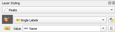
1. In the Layer Styling panel, switch to the Labels tab ![]() .
Switch from No Labels to Single labels. Set the Label with option to the
.
Switch from No Labels to Single labels. Set the Label with option to the Name field.
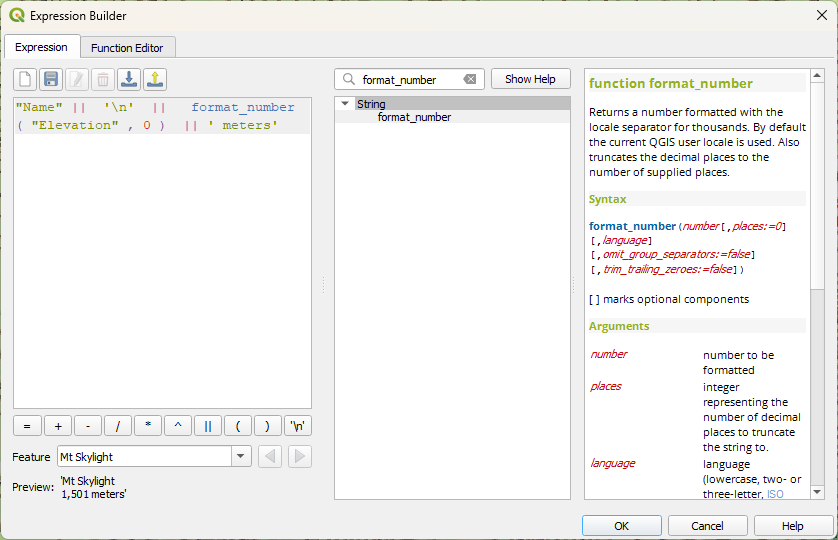
It is also possible to use multiple fields in a feature label by using an expression.
2. Click the Expression ![]() button
to open the Expression Dialog window. Expand the Fields and Values section and add the Elevation field after the Name field. When combining text elements in an expression they need to be separated by the String Concatenation
button
to open the Expression Dialog window. Expand the Fields and Values section and add the Elevation field after the Name field. When combining text elements in an expression they need to be separated by the String Concatenation ![]() operator.
operator.
3. Additionally, the New line ![]() operator can be used to wrap the
new column onto a second line. However, it requires another String Concatenation operator after it. Set up an expression like this
operator can be used to wrap the
new column onto a second line. However, it requires another String Concatenation operator after it. Set up an expression like this "Name" || '\n' || "Elevation".
This is nice but it may not be clear what the number represents and the labels will be easier to read with a thousands separator.
4. To add units of measure to the elevation, you can add the string meters after the value by appending || ' meters' to the existing expression. To accomplish the second enhancement you will use the format_number function. Use the search box to find the format_number function. Insert it right before the "Elevation" field. The help panel will show you the syntax for this function. It requires a number and a number of decimal places.
The number will be the "Elevation" field and the number of places 0. This will simply format the data to a number and insert a thousands separator. Note that we use double quotes for fields and single quotes for normal text
(strings).
5. To make the labels easier to read change the font Style to Bold. Switch to the Label buffer tab ![]() and check the Draw text buffer option. To give more separation between the labels and the feature icon switch to the Label placement
and check the Draw text buffer option. To give more separation between the labels and the feature icon switch to the Label placement ![]() tab and set the Distance to 2 mm.
tab and set the Distance to 2 mm.
6. Finally click the Automated placement settings ![]() button to open the Automated Placement Engine settings. Uncheck the box for Allow truncated labels on edges of map option. This will prevent labels from being cut off.
button to open the Automated Placement Engine settings. Uncheck the box for Allow truncated labels on edges of map option. This will prevent labels from being cut off.
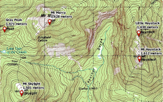
Your labels should now look like:
Watch this video to check the steps for styling and labeling the points:
10.3. Style Rivers
Next you will style the rivers.
1. Set the target layer in the Layer Styling Panel to Rivers and switch from the Labeling tab back to the Styling tab  .
.
2. Select Simple line. Click the Color bar to open the Select line color panel.
3. Change the Color to an RGB value of 31|120|180.
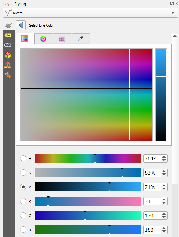
4. Click the Go back ![]() button to return to the main symbology panel.
button to return to the main symbology panel.
5. Increase the Stroke width to 0.86 millimeters.
6. To label the rivers switch to the Labels tab ![]() .
.
7. Repeat the initial steps of labeling Peaks to label Rivers with just the Name field.
8. Switch to the Label placement ![]() tab and choose under
Mode for Curved.
tab and choose under
Mode for Curved.
To make them more readable against the topo map you will apply a buffer.
9. Switch to the Label buffer tab ![]() and check Draw text buffer option.
and check Draw text buffer option.
You will set the color to the green background of the topo map.
11. Click the drop-down arrow for the Color setting and choose Pick color. With the eye dropper cursor click on a place to select that green topo map background color (make sure to select a pixel that is representative for the background color and not a bright green).
12. Finally return to the Text tab ![]() and set the label Color to an RGB value of
and set the label Color to an RGB value of 31|38|180, the Font to Calibri, the Size to 11 and the Style to italic.
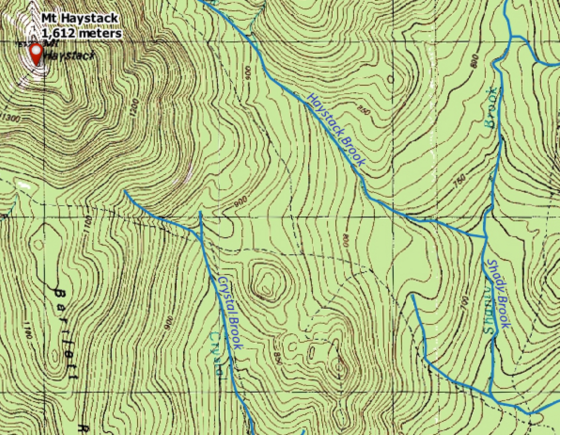
Your rivers should look like:
Watch this video to check the steps of this section:
10.4. Style Lakes
Next you will style the lakes. You will use a shapeburst fill which will allow you to color the lakes from light blue to dark blue.
1. Set the target layer in the Layer Styling Panel to Lakes and switch from the Labeling tab back to the Styling tab.
2. Select the Simple fill styling component. Change the Symbol layer type to Shapeburst fill. Keep the default Gradient colors setting of Two color. Set the first color to an RGB value of 185|239|255.
Set the second color to an RGB value of 31|133|180.
3. Set the Shading style to Set distance with a value of 6. Increase the Blur strength to 12.
Finally you will add a simple line to represent the coastline of each lake.
4. Click the Add symbol layer ![]() button. Change the new Simple fill renderer to a Symbol layer type of Outline: simple line with Color of
button. Change the new Simple fill renderer to a Symbol layer type of Outline: simple line with Color of 31|133|180.
5. Label the lakes with the the Name. Set the label Color and RGB value of 225|255|255 (white), the Font to Calibri, the Size to 10 and the Style to bold italic.
6. Switch to the Label placement ![]() tab and change the
Mode to Horizontal. Then switch to the label Formatting
tab and change the
Mode to Horizontal. Then switch to the label Formatting ![]() tab
and enter a space as the Wrap on character. Set the Alignment to Center.
tab
and enter a space as the Wrap on character. Set the Alignment to Center.
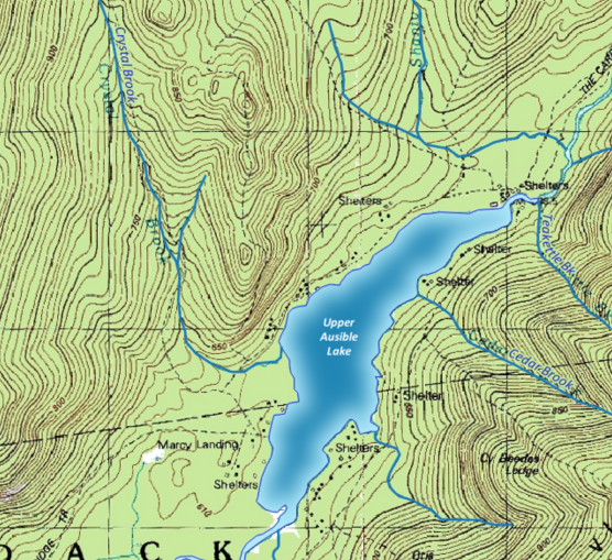
Your lakes should look like:
Watch this video to check the steps in this section:
11. Conclusions
In this lesson you have learned to:
- find the projection and EPSG code of a map
- install plugins
- georeference a scanned map using GCPs from a grid
- use the coordinate capture tool
- use online layers from the QuickMapServices plugin
- digitize points, lines, and polygons and add attributes
- use the snapping toolbar
- dissolve features
- store data in a GeoPackage
- style and label vectors