شاهد هذا الفيديو حول معالجة البيانات الشبكية في نظم المعلومات الجغرافية وأجب عن الأسئلة أدناه.
درس تعليمي: التحليل المكاني باستخدام جبر الخرائط
| الموقع: | OpenCourseWare for GIS |
| المقرر: | تطبيقات في الهيدرولوجيا باستخدام QGIS |
| كتاب: | درس تعليمي: التحليل المكاني باستخدام جبر الخرائط |
| طبع بواسطة: | Guest user |
| التاريخ: | الجمعة، 26 يونيو 2026، 4:09 PM |
1. مقدمة
يتيح لنا جبر الخرائط القدرة على إجراء عمليات حسابية باستخدام الطبقات النقطية. وهذا مفيد في عمليات التحليل المكاني. فعلى سبيل المثال، يمكننا استخدام جبر الخرائط عندما نحتاج إلى تقييم معايير مختلفة لإيجاد مواقع ملائمة أو غير ملائمة.
الأهداف التعليمية
بعد هذا الدرس ستكون قادراً على:
- استخدام جداول خصائص البيانات النقطية (Raster attribute tables).
- تطبيق جبر الخرائط (Map algebra) لإجراء التحليل النقطي.
- التمييز بين البيانات النقطية المنطقية (Boolean)، و المنفصلة (Discrete)، والمستمرة (Continuous).
- إنشاء مفاتيح الخرائط (Legends) للخرائط المنطقية والمنفصلة والمستمرة .
- فهم استخدام قيم Nodata (انعدام البيانات).
- إستخدام المعاملات المنطقية (Logical operators).
- حساب المسافات من البيانات النقطية.
- إعادة تصنيف (Reclassify) البيانات النقطية.
- تحويل البيانات النقطية إلى نقاط اتجاهية (Vector points).
- إستخلاص (Sample) قيم البيانات النقطية باستخدام النقاط الاتجاهية.
وصف الحالة
سنتناول في هذا الدرس الحالة التالية:
كَلفتْكَ بلدية واحة Aïn Kju Dzjis (الافتراضية) بتحليل أي الآبارغير ملائمة لسكانها بناءً على الشروط التالية:
الشرط الأول:
يجب أن تقع الآبار ضمن مسافة 150 متراً من المنازل أو الطرق.
الشرط الثاني:
عدم وجود منشآت صناعية أو مناجم أو مكبات نفايات ضمن مسافة 300 متر من الآبار.
الشرط الثالث:
يجب أن يكون عمق الآبار أقل من 40 متراً.
ستستخدم جبر الخرائط لإجراء التحليل المطلوب.
مسار العمل
سيعتمد هذا الدرس مسار العمل التالي :
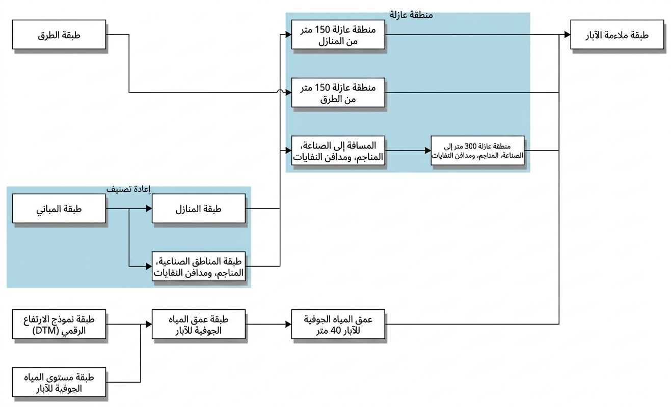
المواد التدريبية
يمكن تحميل الطبقات النقطية الخاصة بهذا الدرس من صفحة الدرس الرئيسية.
2. المادة النظرية
سنعرض أولاً الجانب النظري اللازم لهذا التمرين من خلال عدد من الفيديوهات.
شاهد كل فيديو بعناية وأجب عن الأسئلة الموجودة أسفله.
2.1. معالجة البيانات الشبكية في نظم المعلومات الجغرافية
أسئلة - معالجة البيانات الشبكية
3. تحضير
لهذه المهمة، تم تزويدك بالطبقات النقطية التالية: buildg.tif، roads.tif، dtm.tif وgwlevel.tif.
سنقوم أولاً بفحص البيانات الوصفية لهذه الطبقات، ثم سنقوم بإعداد صندوق أدوات المعالجة (Processing Toolbox) في برنامج QGIS.
3.1. فحص البيانات الوصفية
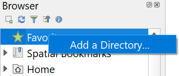
1. في لوحة المتصفح (Browser panel)، انقر بزر الماوس الأيمن على المفضلات (Favorites) واختر Add a directory (إضافة مجلد).
2. إختر المجلد الذي قمت بتخزين الطبقات فيه.
من خلال إضافة مجلد إلى المفضلات، يمكنك الوصول إلى ملفات مشروعك بشكل أسرع.
3. انقر على المثلث الصغير لتوسيع محتويات المجلد.
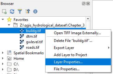
4. قم بمعاينة الخرائط والبيانات الوصفية لهذه الطبقات النقطية من خلال النقر بزر الماوس الأيمن على الطبقة واختيار Layer Properties (خصائص الطبقة)...
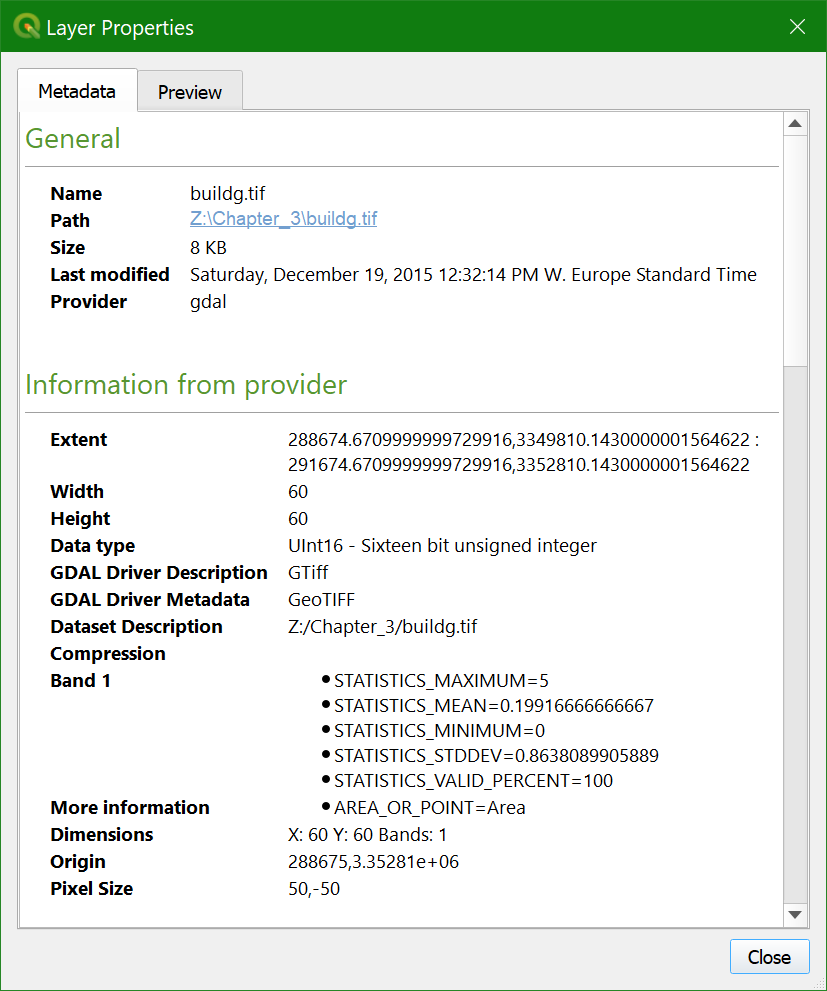
أسئلة - البيانات الوصفية
5. حدد buildg.tif و roads.tif و dtm.tif و gwlevel.tif (مع الاستمرار في الضغط على مفتاح Ctrl عند إختيار الطبقات) ثم قم بسحبها إلى مساحة عرض الخريطة.
6. توجه إلى لوحة الطبقات.
3.2. إضافة جداول خصائص البيانات النقطية
طبقات البيانات التقطية، بصفة عامة، لا تملك جدولاً للخصائص. تمثل كل طبقة موضوعاً واحداً، يتم التعبيرعنه بواسطة قيم الخلايا. وأنواع البيانات التقطية الرئيسية هي:
-
البيانات التقطية المنطقية (Boolean): قيم الخلايا فيها هي صفر أو واحد، مما يعني "صح" أو "خطأ". ومن أمثلتها المناطق المغمورة بالمياه مقابل المناطق غير المغمورة. ويتم تنسيقها باستخدام أداة عرض "القيم الفريدة/الموضحة" (Paletted/Unique values).
-
البيانات التقطية المنفصلة (Discrete): قيم الخلايا فيها هي أرقام صحيحة تمثل فئات محددة. ومن أمثلتها خريطة غطاءات الأرض. وتنسق أيضاً باستخدام أداة عرض "القيم الفريدة/الموضحة".
-
البيانات التقطية المستمرة (Continuous): قيم الخلايا فيها هي أرقام حقيقية (عشرية) تمثل التدرجات في المناظر الطبيعية. وتعد شبكات الارتفاع والمتساقطات أمثلة على ذلك. ويتم تنسيقها باستخدام أداة عرض "مفردة النطاق الكاذب" (Singleband pseudocolor).
يتعين على محلل نظم المعلومات الجغرافية تحديد نوع البيانات، لأن هذا النوع لا يخزن عادةً داخل الطبقة التقطية. فمعرفة نوع البيانات ضروري لتطبيق أدوات التحليل الصحيحة ولعرض البيانات التقطية بالتنسيق المناسب.
أصبح برنامج QGIS يوفر الآن إمكانية إضافة جداول خصائص البيانات التقطية أو ما يعرف بـ RATs إلى الطبقات التقطية، مما يمنح الفرصة لإضافة حقول خصائص متعددة لطبقة تقطية واحدة واختيار حقل معين للتنسيق.
سنقوم بإضافة جدول RAT إلى طبقة buildg. الخطوة الأولى هي تطبيق أداة عرض على هذه الطبقة التقطية المنفصلة التي تحتوي على فئات استخدامات الأرض.
1. حدد طبقة buildg في لوحة الطبقات (Layers panel) وافتح لوحة تنسيق الطبقة (Layer Styling panel).
2. اختر أداة عرض "القيم الفريدة/الموضحة" (Paletted/Unique values) وانقر على تصنيف (Classify) لتعيين لون عشوائي لكل قيمة خلية موجودة في الطبقة التقطية.
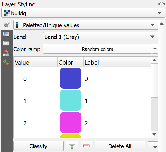
بدون وجود جدول خصائص البيانات الشبكية، يمكاننا تحرير تسميات قيم الخلايا هنا لإنشاء مفتاح للخريطة. أما في هذه الحالة، فسنقوم بذلك داخل جدول RAT.
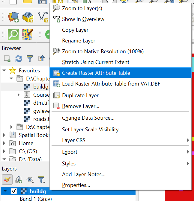
3. في لوحة الطبقات (Layers panel)، انقر بزر الفأرة الأيمن على طبقة buildg واختر Create Raster Attribute Table.
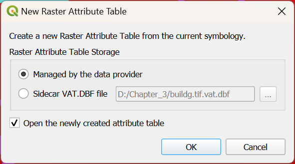
4. في مربع الحوار "جدول خصائص البيانات الشبكية الجديد" (New Raster Attribute Table)، أبقِ على الخيار الافتراضي Managed by the data provider. سيؤدي هذا إلى استخدام صيغة GDAL auxiliary XML. انقر على OK.
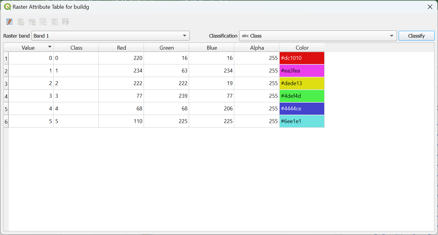
في جدول RAT، ستظهر لك عدة حقول:
- Value: قيم الخلايا الموجودة في الطبقة الشبكية.
- Class: تسمية الفئة.
- RGBA: قيم الأحمر (Red)، والأخضر (Green)، والأزرق (Blue)، وألفا (Alpha - الشفافية) لكل لون من ألوان الفئات.
- Color: الألوان المخصصة للفئات والممثلة بالقيم الست عشرية (Hexadecimal).
كما هو الحال مع جدول الخصائص الاتجاهي، يمكننا أيضًا إضافة حقول إلى جداول RAT (جداول خصائص البيانات النقطية).
-
انقر على زر تحرير جدول الخصائص
 .
. -
انقر على زر عمود جديد
 .
. -
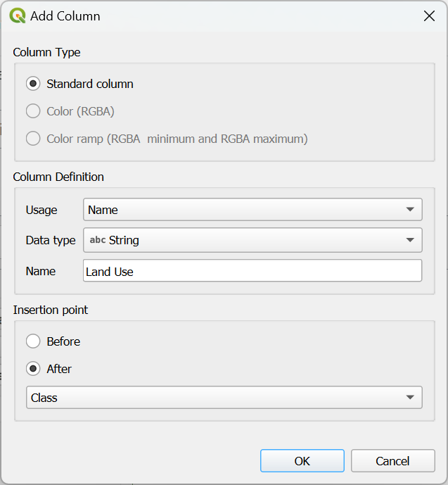
في مربع حوار إضافة عمود جديد (Add new column)، اختر "Usage" للاسم (Name)، و"String" لنوع البيانات (Data type)، واكتب "Land Use" لاسم العمود. وبالنسبة لنقطة الإدراج (Insertion point)، اختر بعد عمود الفئة (After the Class column). انقر على OK.
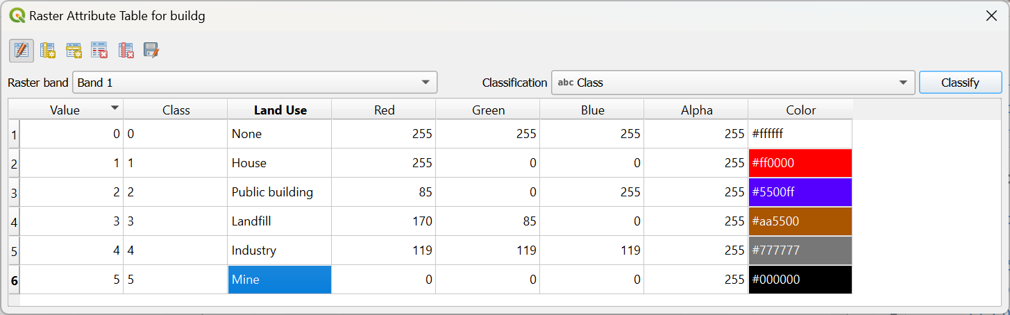
- اكتب أسماء فئات استخدامات الأراضي في حقل Land Use الجديد كما هو موضح أدناه:
-
قم بتغيير ألوان فئات استخدامات الأراضي إلى ألوان أكثر تعبيراً وتلقائية. يمكنك القيام بذلك عن طريق النقر على لون في حقل Color.
-
قم بتغيير حقل التصنيف (Classification) إلى Land Use وانقر على Yes في النافذة المنبثقة لتأكيد رغبتك في استبدال التصنيف السابق.
-
احفظ التعديلات بالنقر على زر Edit Attribute Table مرة أخرى، وانقر على Yes في النافذة المنبثقة لتأكيد حفظ التغييرات.
-
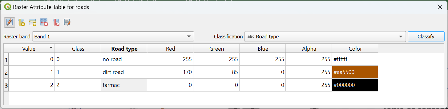
كرر الخطوات لطبقة الطرق (roads) مع الفئات التالية:
0: لا توجد طرق
1: طريق ترابي
2: طريق معبد (إسفلت)
يجب أن تظهر النتيجة كما يلي:
يمكنك أيضاً إنشاء جداول RAT من البيانات النقطية المنسقة باستخدام أداة عرض "مفردة النطاق الكاذب". حينها سيتعين عليك تغيير إعداد "الاستيفاء" (Interpolation) إلى "منفصل" (Discrete) لكي يتم استخدام نطاقات الفئات.
شاهد هذا الفيديو للتحقق من الخطوات في هذا القسم:
3.3. إستخدام تجهيز الأدوات
يوفر صندوق أدوات المعالجة (Processing Toolbox) في برنامج QGIS الكثير من الأدوات لمعالجة بيانات نظم المعلومات الجغرافية. وبالإضافة إلى أدوات QGIS، فإنه يضم أيضاً أدوات معالجة من أطراف خارجية مفيدة جداً؛ ومن الأمثلة عليها: GDAL وGRASS وSAGA وPCRaster Tools وR وWhiteboxTools.
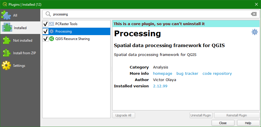
1. يمكنك تفعيل صندوق أدوات المعالجة من خلال اختيار Processing | Toolbox من القائمة الرئيسية.
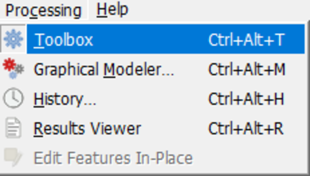
ستظهر الآن لوحة صندوق أدوات المعالجة (Processing Toolbox). ستحتاج إليها في الأقسام التالية.
إذا لم تتمكن من العثور على صندوق أدوات المعالجة في القائمة، فسيتعين عليك تفعيل إضافة Processing في مدير الإضافات (Plugins manager) عن طريق تحديد المربع الخاص بها.
4. الشرط الأول: آبار تقع ضمن 150 متر من المنازل أو الطرق.
بعد أن قمنا بفحص البيانات الوصفية لطبقات الإدخال لدينا وقمنا بإعداد صندوق أدوات المعالجة، حان وقت تحليل الشروط الثلاثة:
- الشرط الأول: آبار تقع ضمن مسافة 150 مترًا من المنازل أو الطرق.
- الشرط الثاني: عدم وجود صناعة أو منجم أو مكب نفايات ضمن مسافة 300 متر من الآبار.
- الشرط الثالث: آبار يقل عمقها عن 40 مترًا.
بالنسبة للشرط الأول، سننظر أولاً في المنازل وسنقوم بما يلي:
- إنشاء طبقة منطقية (boolean) تكون فيها القيمة "صح" (True) للمنازل و"خطأ" (False) للمباني الأخرى.
- إنشاء مناطق (Buffer) بمسافة 150 مترًا حول المنازل. بعد ذلك، سنكرر هذه الخطوات بالنسبة للطرق.
4.1. أنشئ طبقة منطقية تكون فيها القيمة "صح" للمنازل و"خطأ" للمباني الأخرى
إذا أردنا إنشاء طبقة منطقية (Boolean) تكون فيها القيمة "صح" (1) للمنازل و"خطأ" (0) للفئات الأخرى في طبقة buildg، فيمكننا استخدام حاسب البيانات النقطية (Raster Calculator).
-
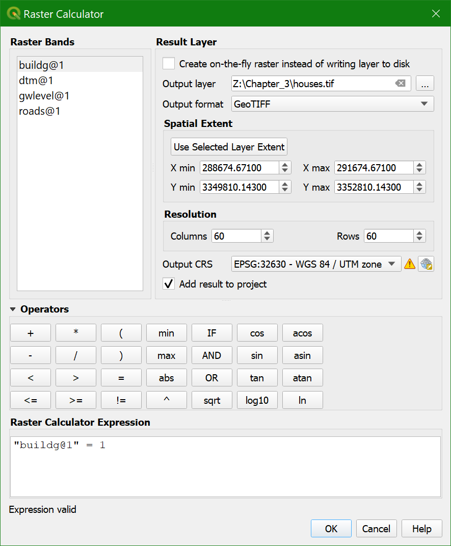
من القائمة الرئيسية، انتقل إلى نقطية | حاسب البيانات النقطية (Raster | Raster Calculator).
-
في نافذة حاسب البيانات النقطية، انقر نقرًا مزدوجًا على buildg@1، ثم انقر على زر = واكتب 1.
تظهر المعادلة الآن كالتالي: buildg@1 = 1، ومعناها: إذا كانت قيمة الخلية في طبقة buildg@1 تساوي 1 (وهي فئة المنازل)، فستأخذ الخلية المقابلة في الطبقة الناتجة القيمة "صح" (القيمة 1)، وإلا فستأخذ القيمة "خطأ" (القيمة 0). ترمز @1 إلى النطاق 1 (Band 1). في حالتنا هذه، نستخدم فقط طبقات نقطية ذات نطاق واحد. (بينما تُستخدم النطاقات المتعددة في تطبيقات أخرى مثل الاستشعار عن بعد).
-
سمِّ طبقة المخرجات باسم houses.tif وانقر على OK لإجراء العملية الحسابية.
-
اتباعاً للممارسات الجيدة، سنقوم بتنسيق هذه الطبقة المنطقية (Boolean). بالنسبة للطبقات المنطقية، نستخدم أيضاً أداة عرض "القيم الفريدة/الموضحة".
شاهد هذا الفيديو للتحقق من الخطوات في هذا القسم:
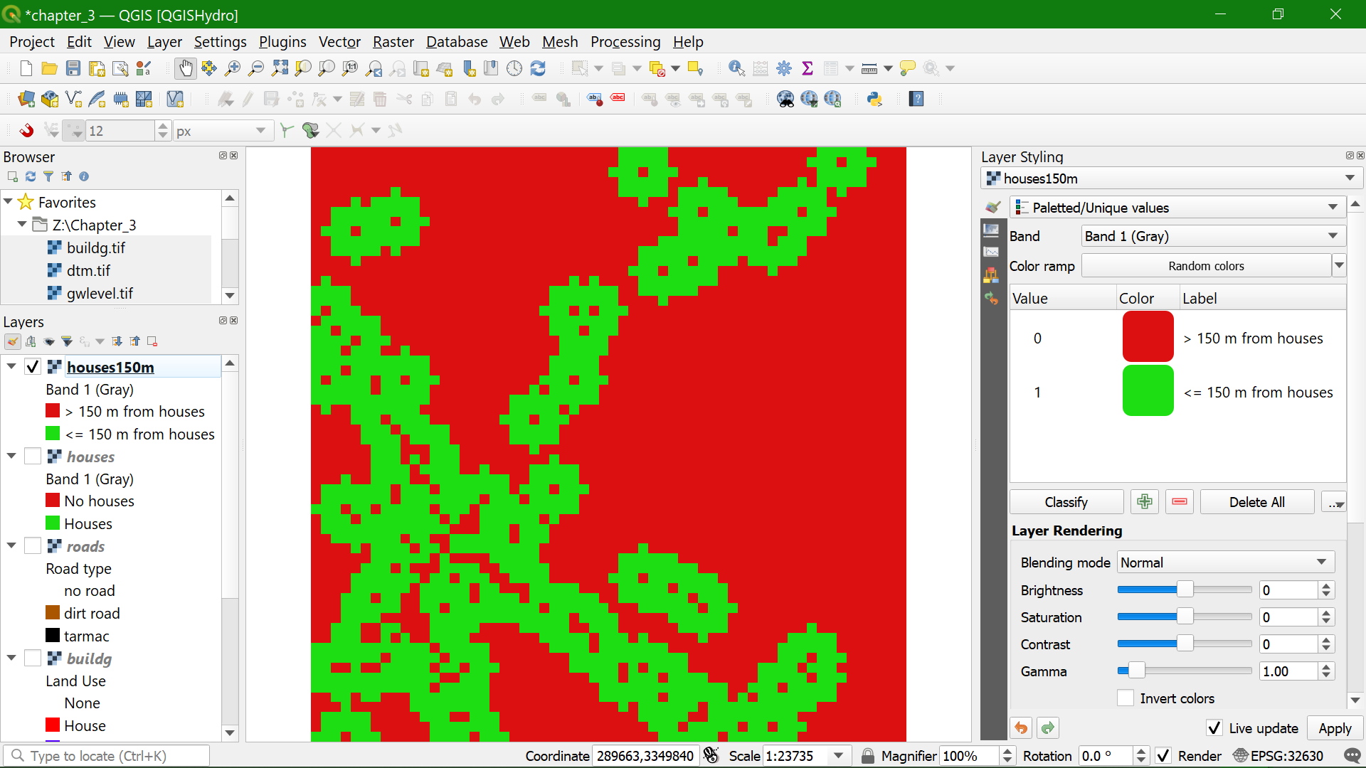
4.2. إنشاء مناطق بمسافة 150 مترًا حول المنازل
بما أننا نملك الآن طبقة تحتوي على المنازل فقط، يمكننا المضي قدماً في حساب مناطق بمسافة 150 متراً حولها. سنقوم بإنشاء طبقة منطقية تكون فيها القيمة "صح" (1) ضمن منطقة الـ 150 متراً حول المنازل، و"خطأ" (0) للمناطق التي تبعد أكثر من 150 متراً عنها.
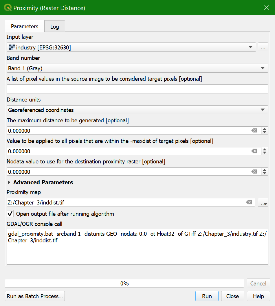
1. من القائمة الرئيسية، انتقل إلى نقطية | تحليل | الاقتراب (المسافة النقطية) (Raster | Analysis | Proximity (Raster Distance)).
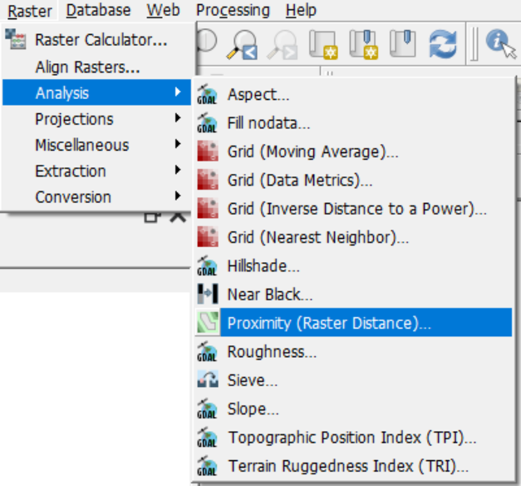
2. في نافذة حوار الاقتراب (المسافة النقطية)، تأكد من اختيار طبقة houses كطبقة إدخال (Input layer). اضبط "وحدات المسافة" (Distance units) إلى الإحداثيات المرجعية الجغرافية (Georeferenced coordinates). وبالنسبة لـ "المسافة القصوى المطلوب توليدها" (Maximum distance to be generated)، أدخل 150 متراً، وأدخل 1 لـ "القيمة التي ستطبق على جميع البكسلات التي تقع ضمن المسافة القصوى (-maxdist) من البكسلات المستهدفة". اضبط "نوع بيانات المخرجات" (Output data type) إلى Byte (لأننا نستخدم فقط 0 و1)، وسمِّ خريطة الاقتراب الناتجة houses150m.tif. اترك الإعدادات الأخرى عند قيمها الافتراضية.
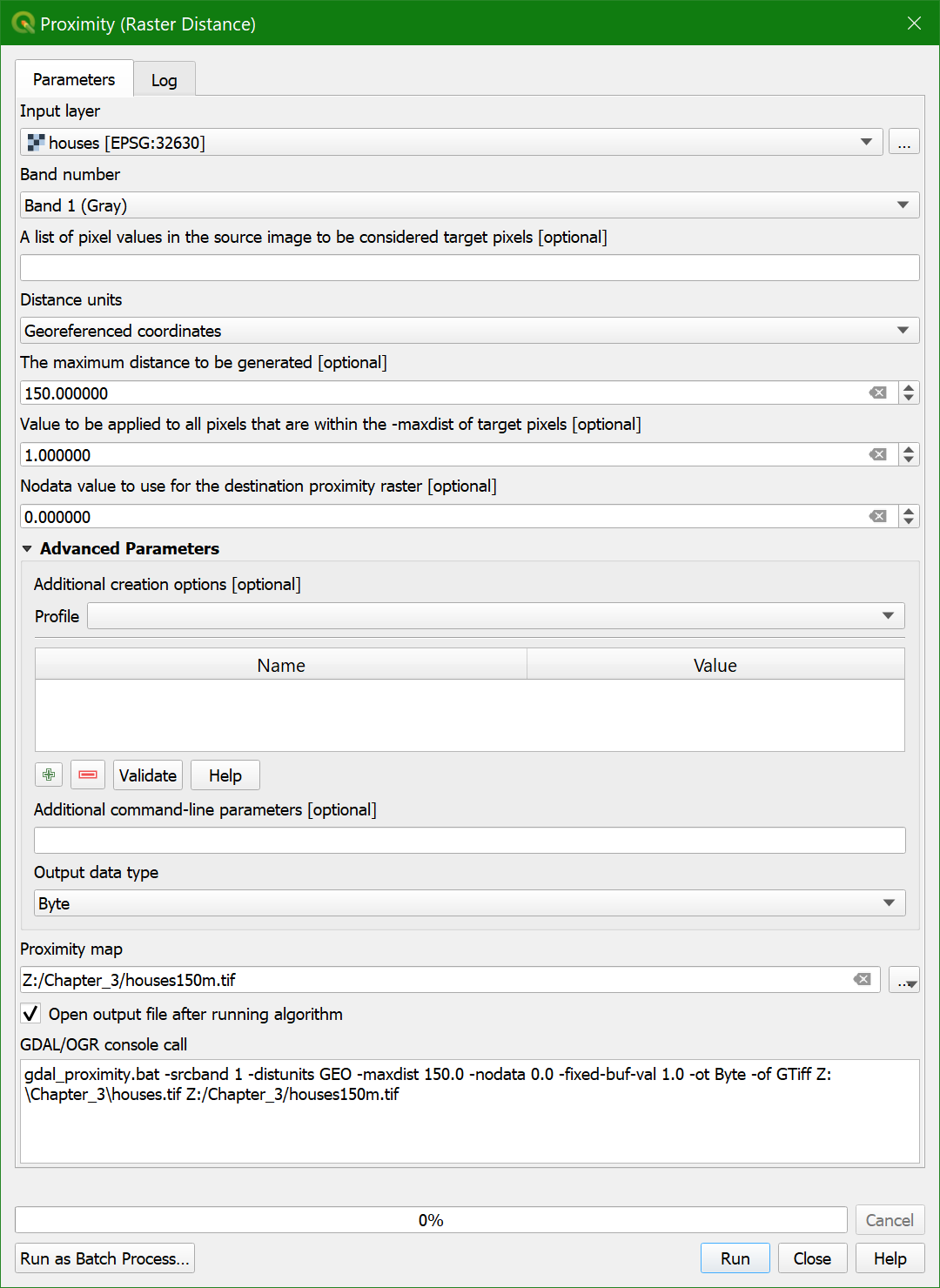
3. أنقر على تشغيل (Run)، ثم إغلاق (Close) عند انتهاء الحساب.
4. نسّق الخريطة المنطقية (Boolean). اجعل البكسلات ذات القيمة "صح" (True) باللون الأخضر، والبكسلات ذات القيمة "خطأ" (False) باللون الأحمر.
شاهد هذا الفيديو للتطلع على خطوات هذا الجزء :
4.3. إنشاء مناطق بمسافة 150 مترًا حول الطرق
بطريقة مماثلة، يمكننا الآن حساب المصد بمسافة 150 مترًا حول الطرق.
1. كرر الخطوات المستخدمة لحساب مناطق الـ 150 مترًا حول المنازل، ولكن استخدم طبقة roads كطبقة إدخال وسمِّ المخرجات roads150m.tif.
2. نسّق الخريطة المنطقية. اجعل البكسلات ذات القيمة "صح" (True) باللون الأخضر، والبكسلات ذات القيمة "خطأ" (False) باللون الأحمر.
5. عدم وجود صناعة أو مناجم أو مكبات نفايات ضمن مسافة 300 متر من الآبار
بالنسبة للشرط الثاني، نحتاج أولاً إلى إعادة تصنيف طبقة buildg بحيث تكون النتيجة خريطة منطقية تأخذ القيمة "صح" (1) للصناعة والمنجم ومكب النفايات، والقيمة "خطأ" (0) للفئات الأخرى. بعد ذلك، نحتاج إلى حساب المسافة إلى البكسلات ذات القيمة "صح"، وأخيراً حساب البكسلات التي تقع على مسافة أبعد من 300 متر عن الصناعة والمنجم ومكب النفايات.
5.1. Create a Boolean Raster with True for Industry, Mine, and Landfill, and False for Other Buildings
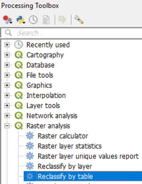
1. From the Processing Toolbox menu choose Raster analysis | Reclassify by table.
The Reclassify table dialogue appears. We are going to reclassify the buildg raster using a lookup table.
2. Fill in the dialog exactly as in the figure below.
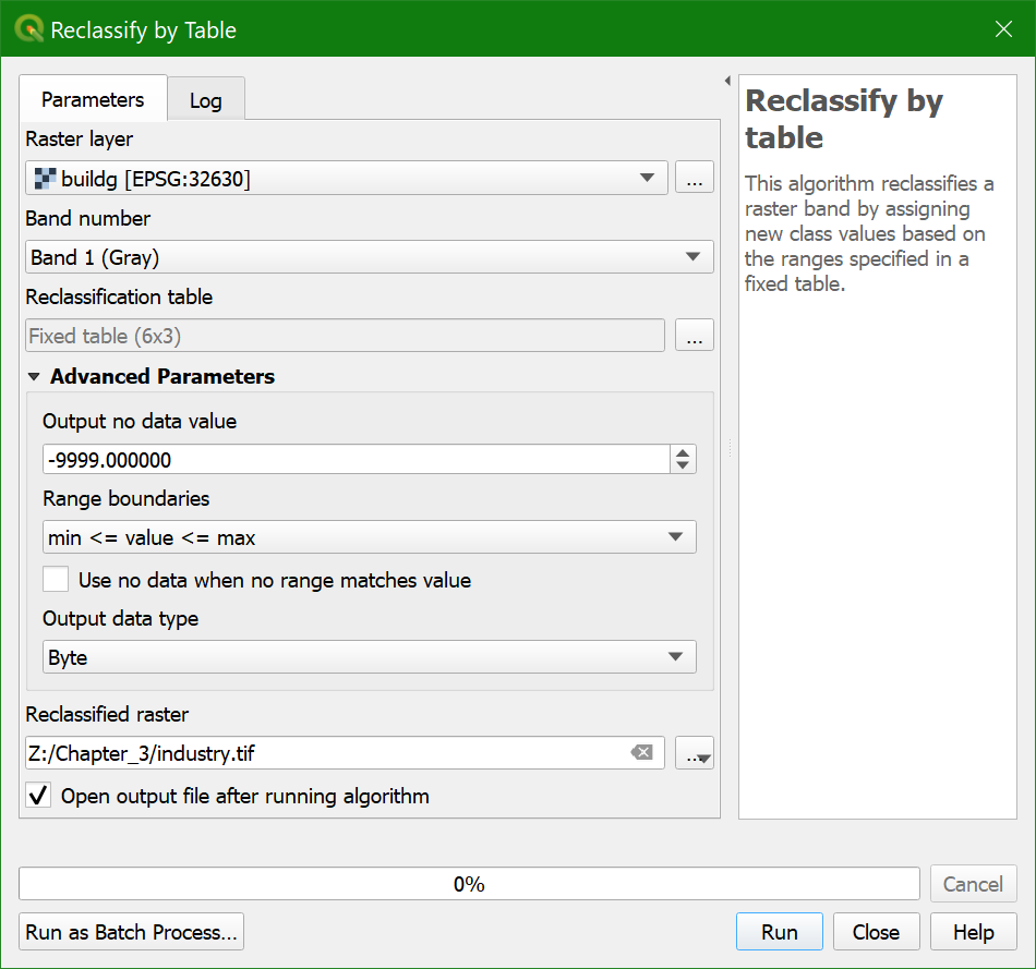
Here you can identify a nodata
value for the output layer for values that are excluded from the lookup table. The Range boundaries define if values are included or excluded from the ranges in a row of the lookup table. Here we don't use ranges, but reclassify each value.
Therefore we choose min <= value <= max. For the Output data type we use Byte because the output values are whole numbers (boolean zero and one) that fit in 8 bits (0-255).
3. Go to Reclassification table and click ![]() .
.
4.
Fill in the lookup table as shown in the figure below.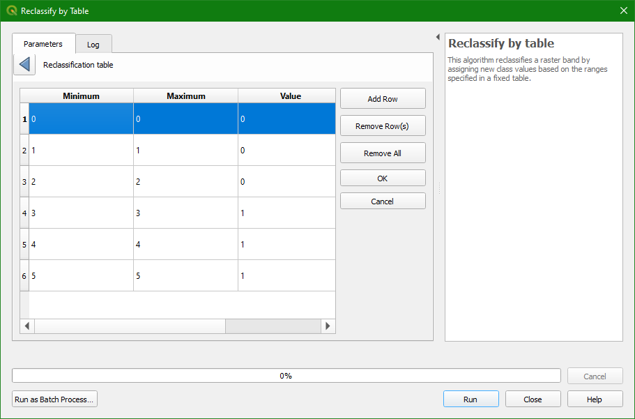
5. Click OK and Run. Close the dialog
when the processing is finished.
6. Check the result: 1 for mines, industry, and landfills, 0 for the other classes. Use the Identify tool ![]() and click on the map. On the lower right panel you can find the identify results. It displays the value of the pixel of the selected layer in the
Layers panel. You might have to resize the columns to see the pixel values.
and click on the map. On the lower right panel you can find the identify results. It displays the value of the pixel of the selected layer in the
Layers panel. You might have to resize the columns to see the pixel values.
- Is industry a boolean, discrete, or continuous raster?
7. Style the industry layer.
Note that we could get the same result using the Raster Calculator.
- Which expression would you have used for this in the Raster Calculator?
Watch this video to check the steps in this section:
5.2. Create Zones of 300 Meters Around Industry, Mine, and Landfill
With the boolean map with True for industry, mine, and landfill we can calculate the distance to these pixels. Because the Proximity (Raster Distance) tool does not allow us to assign values for pixels larger than a threshold, we have to calculate
all distances and then use the Raster Calculator to calculate a boolean map with True for pixels further than 300 meters from industry, mine, and landfill.
1. Open the Proximity (Raster Distance) tool.
2. Make sure
that Industry is the Input layer. Keep all other settings as default. Name the Output proximity map inddist.tif.
3. Check the result.
- Is the inddist layer a boolean, discrete, or continuous raster?
4. Make a legend that is appropriate for this raster type using Singleband pseudocolor as the render type. Use intuitive colors (e.g. a ramp from red to green).
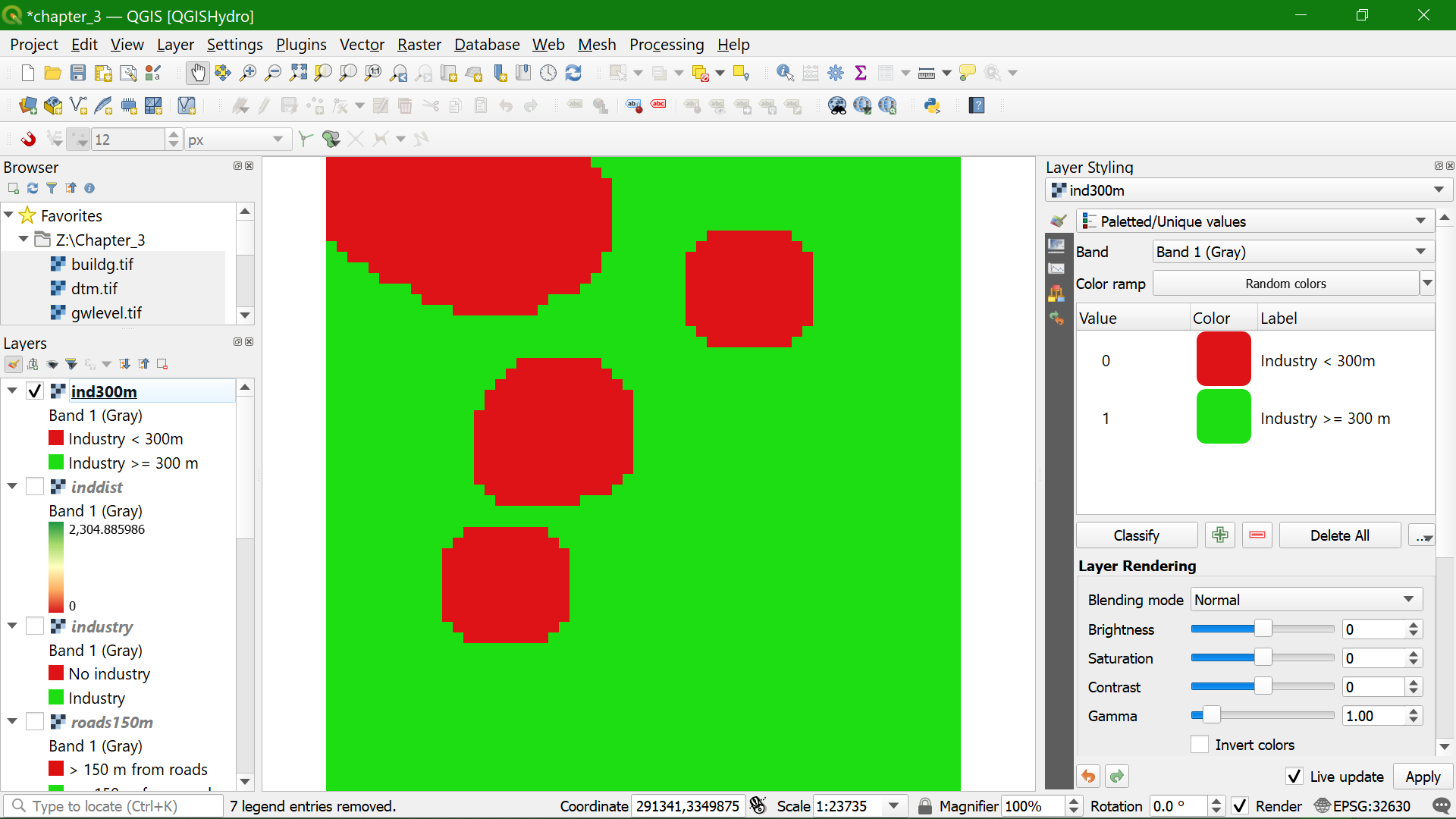
5. Use the Raster Calculator to calculate inddist@1 >= 300.
Call the output layer ind300m.tif.
- Is the ind300m layer a boolean, discrete, or continuous raster?
6. Style the ind300m layer.
Watch this video to check the steps in this section:
6. Condition 3: Wells Less than 40 Meters Deep
For the last condition we need to identify the wells that are less than 40 m deep.
The gwlevel layer gives the absolute elevation of the groundwater level in the well in meters above sea level. In order to calculate the depth to the groundwater, we need to subtract this from the surface elevation given in the digital terrain
model (DTM).
1. Open the Raster Calculator.
2. Subtract the absolute well depth from the DTM using this calculation: dtm@1 - gwlevel@1. Call the output layer welldepth.tif.
- Is the welldepth layer a boolean, discrete, or continuous raster?
3. Style the welldepth layer with the appropriate renderer for this raster type.
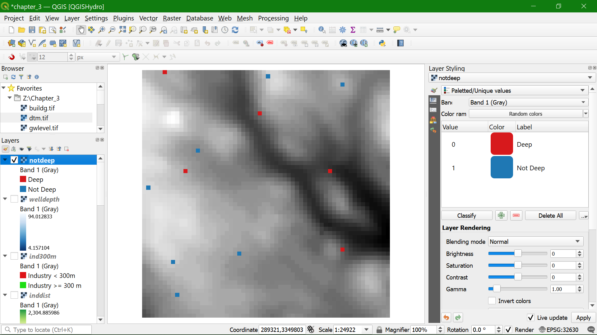
4. Next, calculate in the Raster Calculator a boolean map with wells less than 40 m deep. Call the output layer notdeep.tif.
5.
Style the notdeep layer.
Watch this video to check the steps of this section:
7. Combine the Three Conditions
After calculating the boolean rasters for the three conditions we need to combine them to come to the final result.
1. Use the Raster Calculator to combine the three conditions. Because all boolean results for the conditions need to be True we have to use the AND operator. Call the output layer accessiblewells.tif.
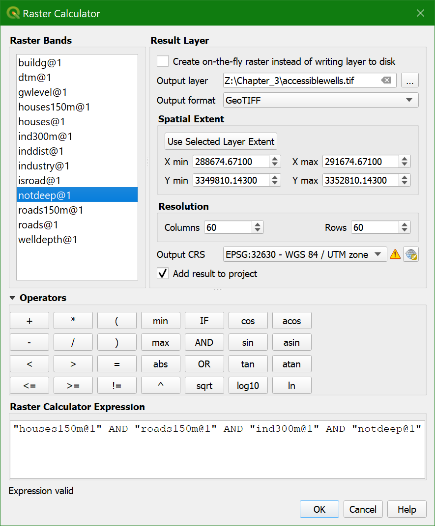
2. Check the resulting
raster layer and style the layer.
Watch this video to check the steps of this section:
8. Report the results
Now we have identified the accessible and inaccessible wells we need to prepare the result map for reporting to the contractor.
In the next steps, we are going to:
- Convert raster cells of the wells to point vectors for a better visualisation
- Sample raster values to add attributes from the calculated layers
- Style the analysis results
8.1. Convert Raster Cells to Point Vectors
To present the end result, we can style the accessiblewells layer. However, it is nicer to present the wells as point features on the map. Therefore, we need to convert the well pixels to point vectors.
1. In the Processing Toolbox go to Vector creation | Raster pixels to points.
![]()
2. In the dialog choose
the accessiblewells layer as the input Raster layer. For Field name, enter Accessible. The raster values will be saved under this field in the attribute table. Choose wells.shp as the output Vector points layer.
![]()
3. Click Run,
then Close when the conversion is finished.
Watch this video to check the steps in this section:
8.2. Sample Raster Values
The point vector layer wells now only contains the field Accessible. It is however, more informative to also include other data in the attribute table. With the Point sampling tool plugin we can sample the raster layers in this project
and add that information to the point attribute table.
1. Install the Point sampling tool plugin.
2. In the Layers panel only check the boxes before the layers you want to sample and uncheck the others. Choose the following
layers: dtm, welldepth, gwlevel, notdeep, ind300m, roads150m, and houses150m.
3. Click the Point sampling tool button ![]() .
.
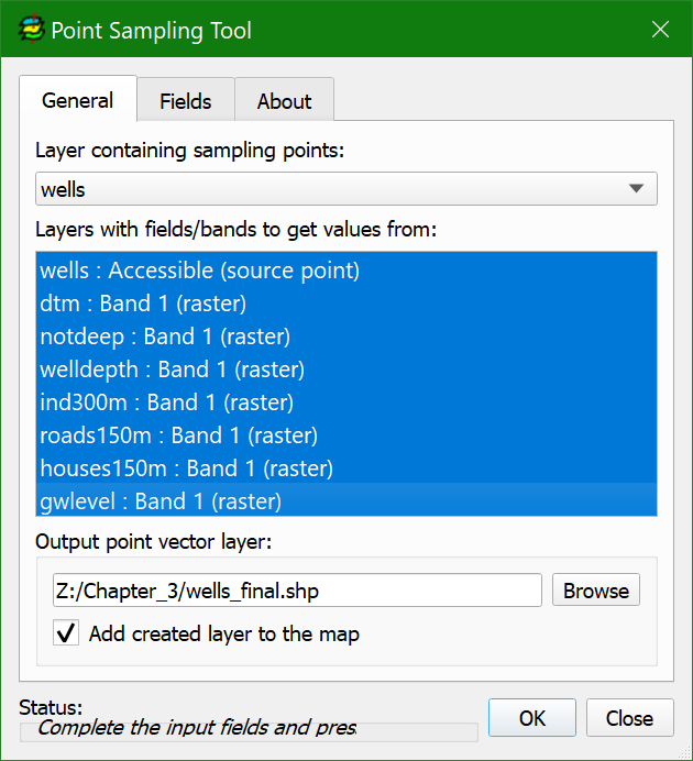
4. In the General tab of the Point Sampling Tool dialog choose wells as the layer containing sampling points,
select all Layers with fields/bands to get values from and save the Output point vector layer to wells_final.shp.
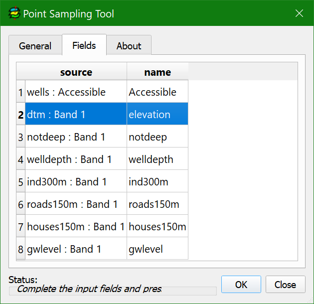
5. Click the Fields tab.
6. Edit the name of the attribute that will be given to the output field if needed.
7. Click OK and
Close.
8. Open the attribute table of wells_final and check the result.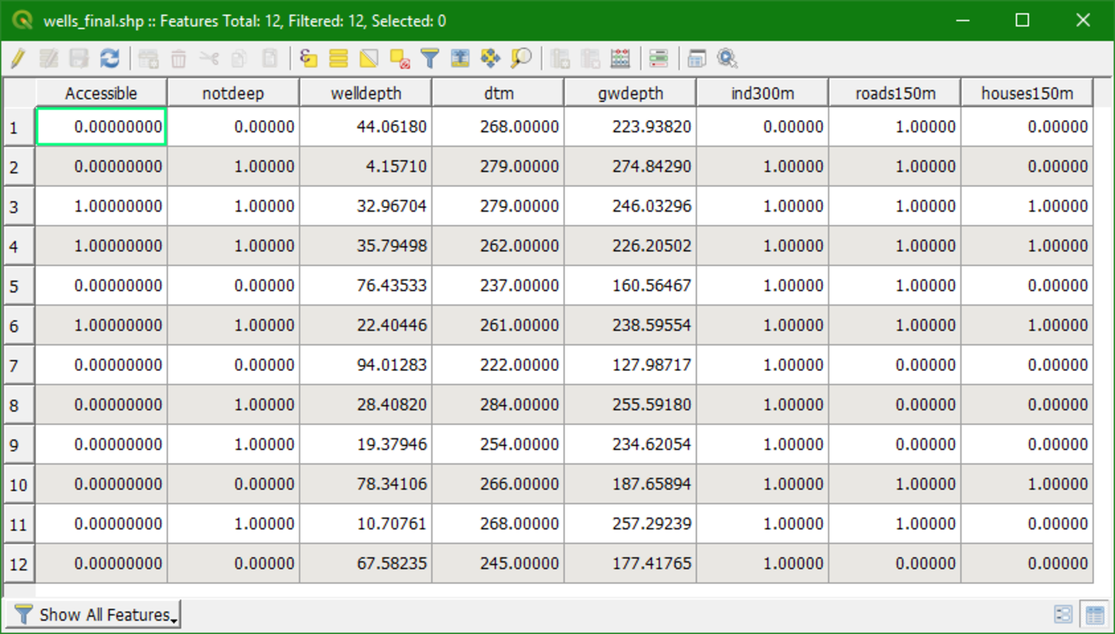
Watch this video to check the steps of this section:
8.3. Style the Analysis Results
Now we can style the layers.
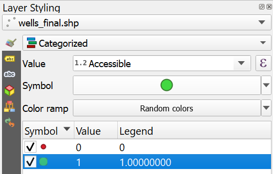
The first step in showing the results will be to style the wells_final data by whether the wells are accessible or not.
1. In the Layers panel, click on the ![]() to open the Layer styling panel. Set wells_final as the target layer.
to open the Layer styling panel. Set wells_final as the target layer.
2. Change from a Single symbol to a Categorized renderer. Then set the Value to Accessible. Click
Classify.
3. When using this renderer QGIS will create a category to capture any NULL values. Here there are no wells with NULL values in the Accessible field. Select the entry where the Value reads all other values and click the Delete ![]() button to remove
it. Give the wells with a value of 1 a green symbol with a size of 4 mm. Give the wells with a value of zero a red color with a size of 2 mm.
button to remove
it. Give the wells with a value of 1 a green symbol with a size of 4 mm. Give the wells with a value of zero a red color with a size of 2 mm.
4. In the Legend column rename the entry with a Value of 1 to Accessible and the entry with a Value of zero to Inaccessible.
5. Scroll down in the Layer styling panel
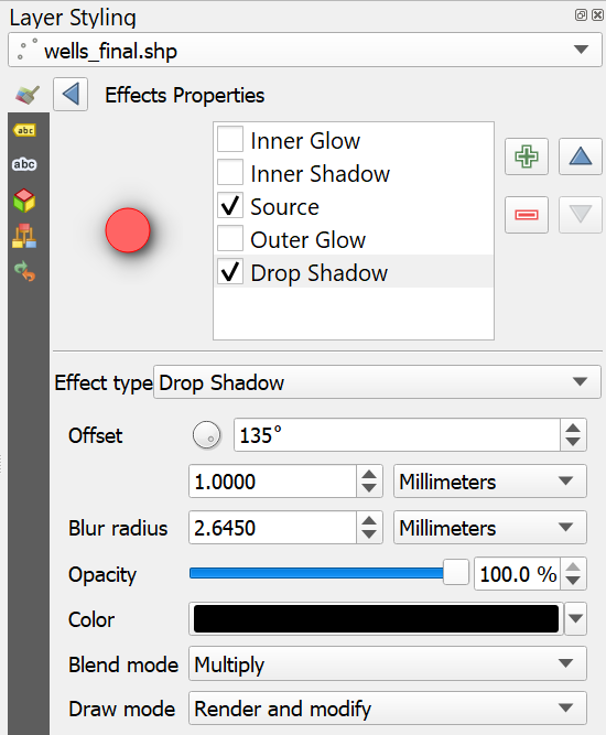
and find the Layer Rendering section. Expand it and select Draw effects. The Customize effects ![]() icon becomes active. Click on it to open the Effects properties panel.
icon becomes active. Click on it to open the Effects properties panel.
Here you can add Inner and Outer Glows, Drop Shadows, and other effects.
6. Click the box next to Drop Shadow. Select the Drop Shadow effect so that you are seeing the parameters of the Drop Shadow. Reduce the Offset distance to 1.0 mm. Click the Go back ![]() button to return to the main styling panel.
button to return to the main styling panel.
6. Switch to the Labels tab ![]() of the Layer styling panel.
of the Layer styling panel.
7. Change the setting from No labels to Single labels. Set the Label with column to welldepth.
You will use a labeling expression very similar to that used at the end of the "Preparing Data from Hardcopy Maps" chapter where we labelled the peaks. You will set the expression up so the labels read something
like: Well Depth: 76.4 m.
8. Click the Expression ![]() button to open the Expression Dialog window.
button to open the Expression Dialog window.
9. To begin, add the string Well Depth in front of the well depth value by adding 'Well Depth: ' before the existing expression.
10. To
accomplish the second component you will use the format_number function. Use the search box to find the format_number function. Insert it right before the welldepth field. Remember, this function requires a number
and a number of decimal places. The number will be the welldepth field and the number of places 2.
11. Use what you learned about the String Concatenation ![]() operator
and the the New line
operator
and the the New line ![]() operator to
nicely format the label and add the units to the end.
operator to
nicely format the label and add the units to the end.
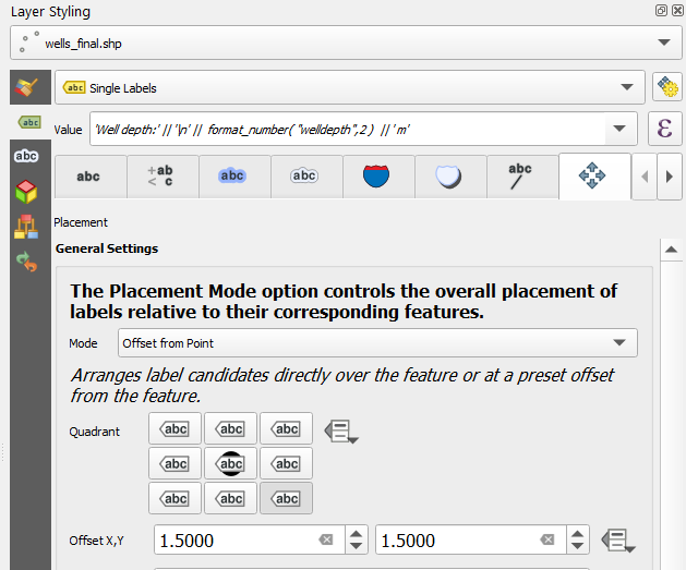
12. Your expression should resemble 'Well Depth:'|| '\n' || format_number(welldepth,2) || ' m'.
13. Set the Font to a sans serif font with a Size of 9 points.
14. Switch to the Placement ![]() tab and choose for Mode Offset from point. Select the lower right Quadrant placement with an Offset X Y setting of 1.5 mm each.
tab and choose for Mode Offset from point. Select the lower right Quadrant placement with an Offset X Y setting of 1.5 mm each.
15. Finally click the Automated placement settings ![]() button to open the Automated Placement Engine window. Uncheck the box for Allow truncated labels on edges of map option.
This will prevent labels from being cut off.
button to open the Automated Placement Engine window. Uncheck the box for Allow truncated labels on edges of map option.
This will prevent labels from being cut off.
16. To complete the styling you will work with the dtm layer. Make this layer the target layer in the Layer styling panel. Choose Singleband pseudocolor as renderer. Click
the drop-down for the Color ramp and choose Create new color ramp.
17. The Color ramp type window opens. Choose Catalog:cpt-city as the type. Click OK.
18. The Cpt-city Color Ramp window will open. Select the Topography category.
19. Choose sd-a and click OK. Click Classify.
Did you know that you can save this color ramp to your style library? To do this access the color ramp context menu and select Save color ramp. The Save New Color Ramp window will open allowing you to give it a Name and provide Tag(s).
20. Scroll down to the Layer Rendering section and set the Blending mode to Mulitply.
21. Finally right-click on the dtm layer and choose Duplicate from the context menu.
22. Rename dtm copy to hillshade (click right on the layer and choose Rename) and
turn it on.
23. Make the hillshade layer the target layer in the Layer styling panel. Change the renderer to Hillshade. Scroll down to the Layer Rendering section and set the Blending mode back to
Normal.
24. In the Resampling section, set Zoomed in to Bilinear to create a smooth visualisation. You can also do this for the dtm layer.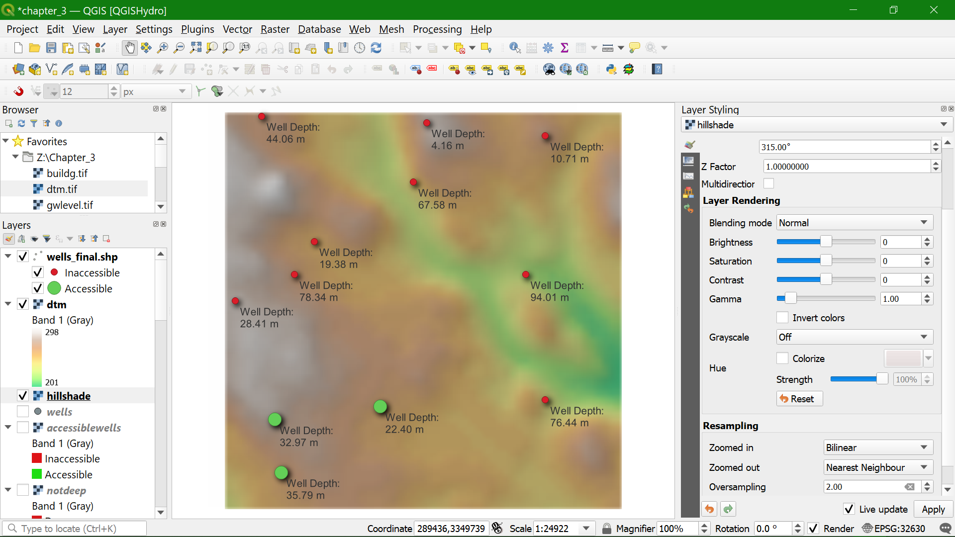
Watch this video to check the steps in this section:
9. Conclusions
In this lesson you have learned to:
- use raster attribute tables
- apply map algebra for raster analysis
- distinguish Boolean, discrete, and continuous rasters
- make legends for Boolean, discrete, and continuous maps
- understand the use of Nodata
- use logical operators
- calculate distances from rasters
- reclassify rasters
- convert raster to vector points
- sample raster values with vector points
You can watch this playlist with all relevant videos for this lesson:
Before proceeding to the next lesson, please submit the assignment of Lesson 3.