Tutorial: Remote Sensing Image Classification with QGIS
| Site: | OpenCourseWare for GIS |
| Disciplina: | Land-Cover Mapping with QGIS |
| Livro: | Tutorial: Remote Sensing Image Classification with QGIS |
| Impresso por: | Guest user |
| Data: | quarta-feira, 15 de julho de 2026 às 02:07 |
1. Introduction
Remote sensing–based land-cover classification is a cornerstone of modern environmental analysis, agricultural monitoring, and land‑use mapping. In this tutorial, you will work hands‑on with QGIS and two powerful open‑source plugins (AI Segmentation Plugin and the Semi‑Automatic Classification Plugin) to build a complete workflow from raw satellite imagery to an evaluated land‑cover map.
Below you'll find what you'll be able to do after completing this tutorial:
Data Preparation & Environment Setup
-
Create a dedicated QGIS profile for remote sensing workflows.
-
Load and organize reference vector data and backdrop layers.
-
Label and structure ground‑truth points for classification.
Segmentation & Training Data
-
Install and configure the AI Segmentation Plugin.
-
Generate parcel‑level segments and split them into training and test areas.
Image Processing & Classification
-
Download Sentinel‑2 imagery using SCP.
-
Construct a band set and clip imagery to a study area.
-
Import, evaluate, and refine training areas.
-
Set up and run a Random Forest classifier.
-
Preview and produce a full‑scene classification.
Validation & Interpretation
-
Perform an accuracy assessment using test data.
-
Interpret classification outputs and identify potential improvements.
2. Create a New QGIS Profile
Before we start, we'll first create a new QGIS profile. A QGIS profile is a self‑contained workspace that stores all your personal QGIS settings, including:
- Installed and enabled plugins
- Toolbar and panel layouts
- Language settings
- Font and icon sizes
- Processing settings
- Color ramps, styles, and favorites
- Authentication settings
- Python console history
- Custom forms and templates
Each profile behaves like its own mini‑QGIS environment. This means you can create different profiles for different tasks, for example, one for cartography, one for teaching, and one for remote sensing.
Some plugins, such as the Semi‑Automatic Classification Plugin (SCP), add many toolbars, panels, and processing providers. They are powerful, but they can also:
- Slow down QGIS startup
- Add visual clutter
- Load tools you don’t need for other workflows
- Conflict with other plugins, resulting in strange Python errors
By creating a dedicated Remote Sensing profile, QGIS will only load the plugins required for that workflow. Your default profile stays clean, and QGIS will start faster because it doesn’t have to load everything.
Tip: When you get strange errors, the first solution is to try if QGIS works again properly in a clean profile. Often conflicting plugins cause errors. Reinstalling QGIS does not solve the problem, because it doesn't replace your profiles!
Let's create a dedicated profile for remote sensing analysis.
- Start QGIS Desktop.
- In the main menu, go to Settings | User Profiles | New Profile....
- Give your profile a simple name without spaces or accents, for example remote_sensing.
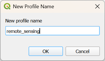
- Click OK.
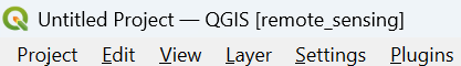
QGIS will now open a new window with your profile.
5. Close the other QGIS window.
From now QGIS will open with your new profile.
At any time, you can switch profiles via the main menu: Settings | User Profiles | [choose profile]
You can identify the current project by its name in square brackets in the upper left of your QGIS window.
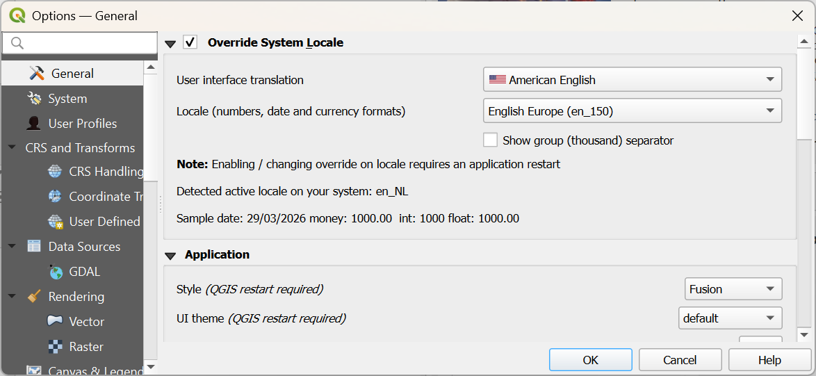
If your QGIS is not in English, you can also change it now for this profile, so the screenshots in the tutorial match with what you see on your computer. You can change the language by choosing in the main menu: Settings | Options.... In the General tab, check the box before Override System Locale and choose the appropriate User interface translation and Locale.
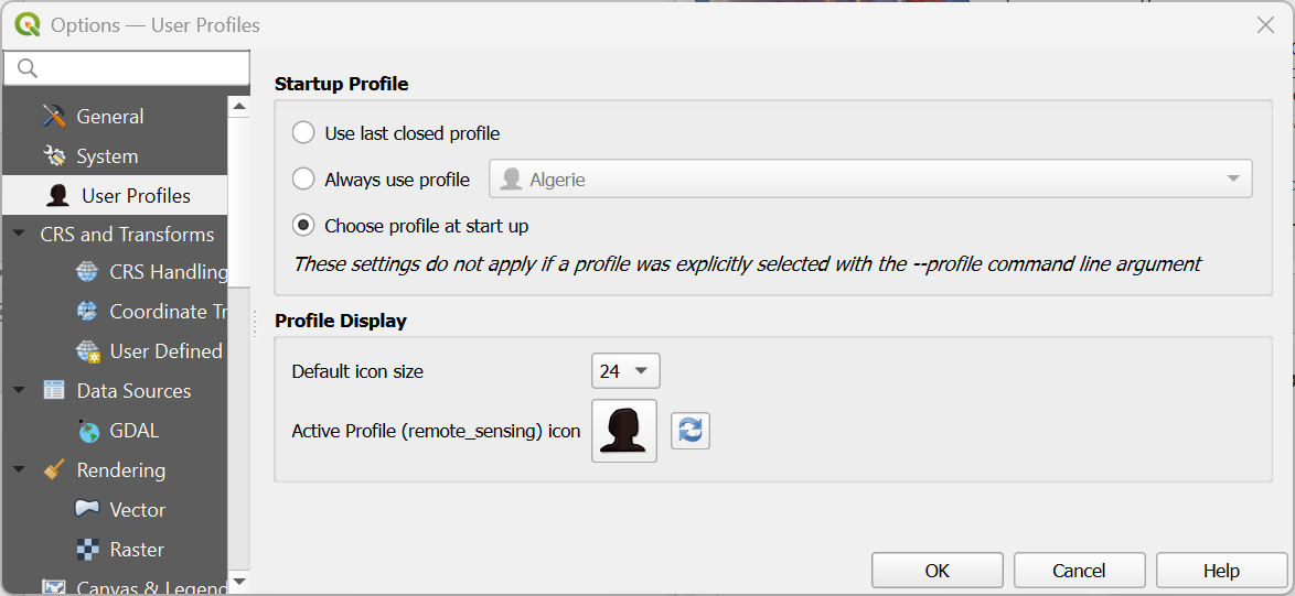
If you have many profiles, you can also use a setting to start QGIS with a popup to let you choose which profile you want to use. You can do this by choosing from the main menu Settings | Options.... Under the User Profiles tab, you can select Choose profile at start up.
More info about setting up profiles in this video:
This video shows how to change language settings:
3. Preparing Ground Truth Data
Before we can train any classification model or even begin segmenting the landscape, we need a solid foundation of ground truth data. In this chapter, we bring together the essential reference layers that will anchor the entire workflow: the study area boundary, the reference points, and a high‑resolution Google Satellite backdrop to support visual interpretation.
These layers form the spatial context in which we will later delineate reference polygons using AI segmentation. B
You will learn how to:
- Load and inspect the reference vector data
- Add the study area boundary to constrain the analysis
- Bring in a Google Satellite basemap to support interpretation
- Add labels to the ground truth points for easier navigation
In the next chapter, we will use this setup to delineate reference polygons, which will later be split into training and test areas for the classification.
3.1. Load Reference Vector Data
Before we can delineate polygons with their class information, we need to load:
- The boundary of the study area
- A point dataset with groundtruth information
- A backdrop from which we can delineate the polygons
The boundary polygon and point dataset can be found in a GeoPackage that you can download here or from the main course page.
- Open QGIS Desktop with an empty project.
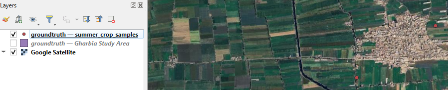
- Go to the Browser panel and locate the GeoPackage file that you have downloaded.
- Drag the Gharbia Study Area and summer_crop_samples layers from the Browser panel to the map canvas.
Note that the ground truth points only cover a part of the Gharbia area. Also note that the project is EPSG:32636, which is UTM Zone 36 North / WGS-84.
Let's inspect the attribute table of the summer_crop_samples.
4. In the Layers panel click right on the summer_crop_samples layer and choose Open Attribute Table from the context menu.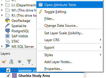
Which land-cover classes are in the ground truth data?
In the next section we'll add a backdrop.
3.2. Load Backdrop Layer
We will assume that the parcel boundaries have stayed more or less the same through time. For delineating the parcels, we could use the same Sentinel-2 image as we will use for the classification. A high resolution satellite image, however, would be more precise.
We'll load a Google Satellite image with the QuickMapServices plugin.
Let's first install the plugin.
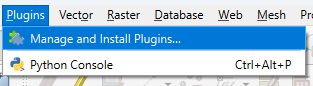
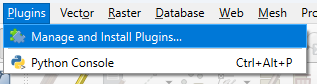
1. In the main menu go to Plugins | Manage and Install Plugins....
2. Search for the NextGIS QuickMapServices plugin and click Install Plugin.
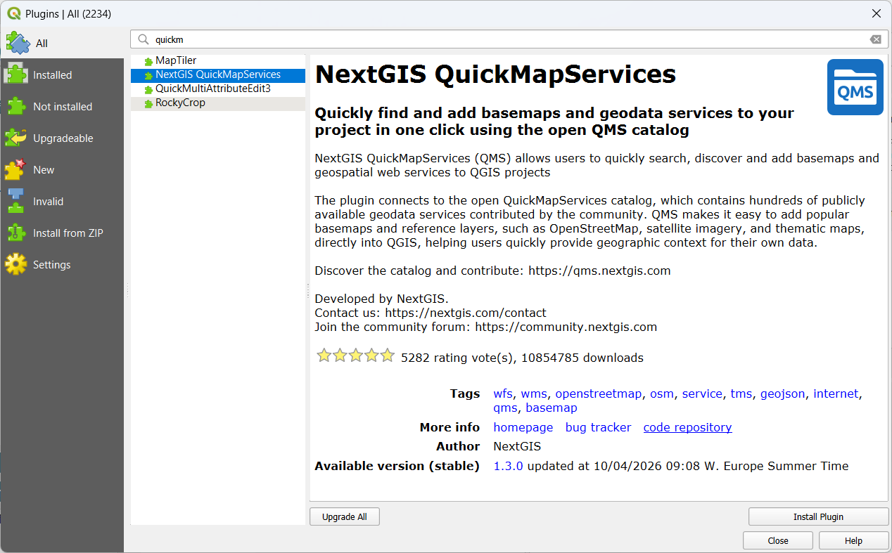
3. Click Close to close the dialog.
Now we can look for the Google Satellite layer and load it into the map canvas.
4. In the main menu, go to Web | QuickMapServices | Google | Google Satellite.
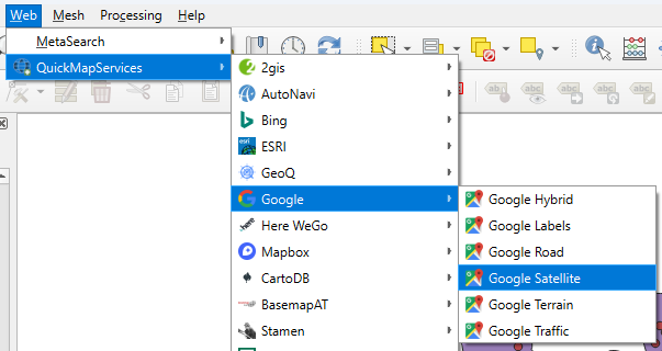
The satellite image is now visible in the map canvas.
In the next section, we'll improve the visibility of the ground truth data on the satellite backdrop.
3.3. Add Labels to Ground Truth Points
Now we have all reference layers in the map canvas, we can improve the visualisation a bit before we can start segmenting parcels.
1. Hide the Gharbia Study Area layer and make sure that the summer_crop_samples layer is on top of the Google Satellite layer.
Later we'll use AI-based segmentation to delineate the parcels belonging to the ground truth points. To make it easier we can label the points with the class name.
2. Select the summer_crop_samples layer and click  to open the Layer Styling panel.
The Layer Styling panel appears, but is partly covered by another panel from the QuickMapServices plugin.
3. Close the Search NextGIS QMS panel by clicking the cross in the upper right of the panel.
4. Go to the Labels  tab.
tab.
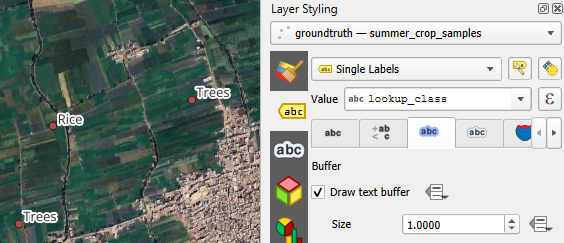
5 From the drop-down menu choose Single Labels.
6. At Value choose the Lookup_class field which has the class names.
The names with the black font are not very visible on the satellite backdrop. Let's improve this by adding a text buffer.
7. Go to the Buffer  tab.
tab.
8. Tick the box before Draw text buffer.
9. Save the project to the GeoPackage with the data layers. In the main menu, go to Project | Save To | GeoPackage....
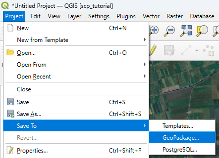
10. Choose the existing GeoPackage and save the project as crop_classification.
Now we're ready to proceed with the AI segmentation.
4. Segment Parcels with the AI Segmentation Plugin
For decades, digitising parcels in remote sensing and GIS workflows meant drawing polygons by hand. Anyone who has traced field boundaries or building footprints knows how time‑consuming this can be. Even with good basemaps, careful snapping, and plenty of patience, manual digitizing remains one of the slowest steps in many mapping projects.
In recent years, however, a new wave of tools has started to transform this process. QGIS now hosts an expanding ecosystem of plugins that use artificial intelligence to automatically segment objects in imagery. Many of these tools build on Meta’s Segment Anything Model (SAM), a foundation model trained on billions of image–mask pairs to identify and outline objects of almost any type, even in images it has never seen before. SAM doesn’t “know” what a parcel or a tree is; instead, it excels at finding coherent shapes and boundaries, making it a powerful engine for geospatial segmentation tasks.
In this chapter, we’ll work with one of the most accessible implementations of this technology: the AI Segmentation plugin by Terralab. It’s lightweight, easy to install, and designed to integrate smoothly into everyday QGIS workflows. With just a few clicks, you can generate clean parcel boundaries from high‑resolution imagery, dramatically reducing the time you spend digitizing.
Watch this video for a quick demo of the plugin:
Let's get started.
4.1. Install the AI Segmentation Plugin
In this section we'll install the AI Segmentation by Terralab plugin.
-
In the main menu go to Plugins | Manage and Install Plugins....
- Search for AI Segmentation by Terralab and click Install Plugin.
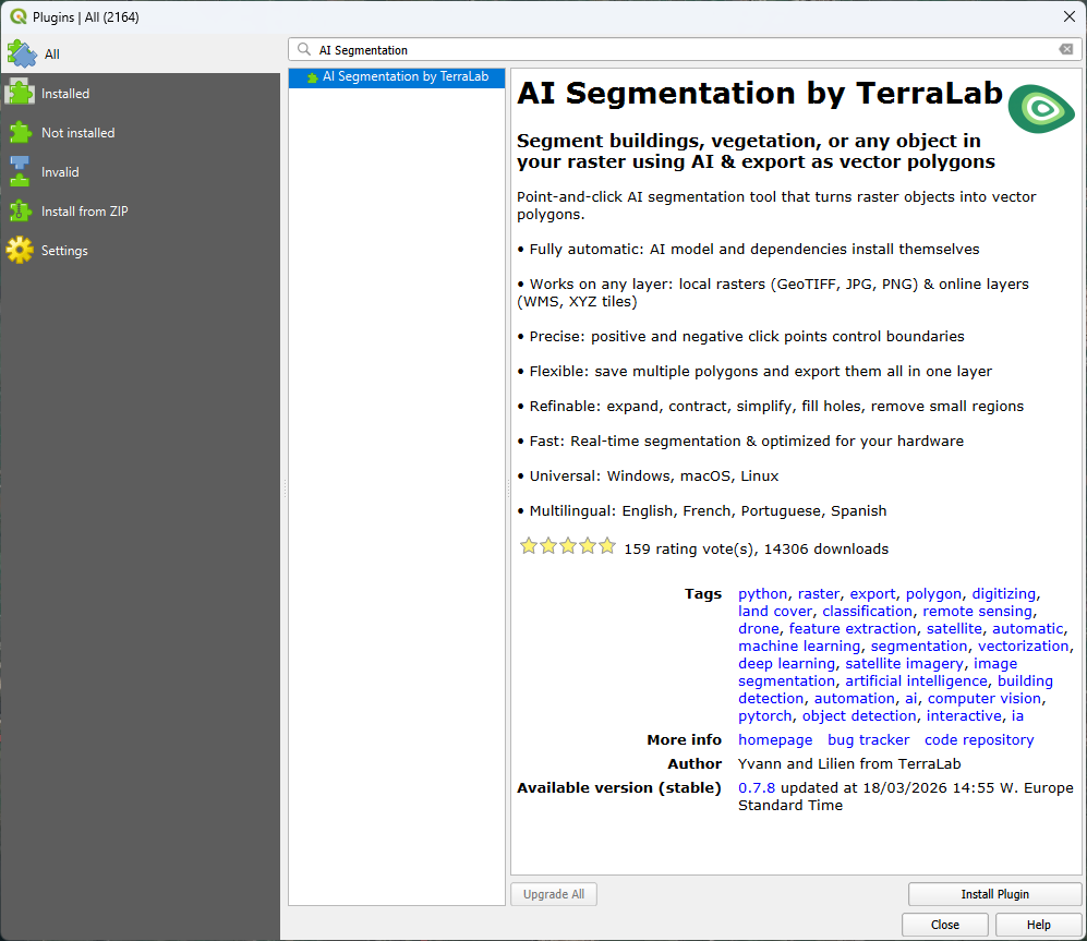
- After installation, click Close to close the dialog.
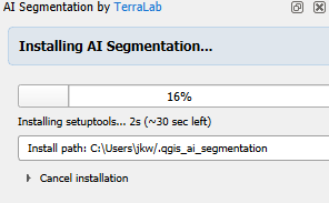
4. In the toolbar, click  to open the panel of the AI Segmentation plugin.
It will start automatically installing the dependencies.
5. Meanwhile, you can register in the popup. Click Get my verification code.
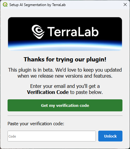
6. A web page will open now. Register with your e-mail address and copy the verification code.
7. Paste the verification code in the dialog and click Unlock.
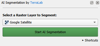
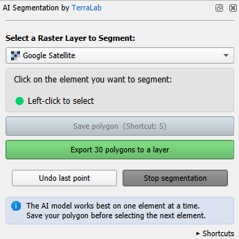
When the installation is completed, the panel looks like the screenshot below.
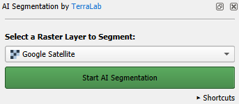
In the next section, we'll start segmenting parcel polygons at our ground truth points.
4.2. Segment Polygons
Now we're ready to segment the parcel boundary polygons with AI and register the class information in the attribute table.
Note that the backdrop is of a different date than our ground truth points, but we assume that the parcels have remained the same.
- Zoom in to a ground truth point.
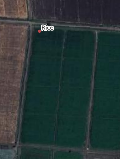
- In the AI Segmentation by TerraLab panel, click on the green Start AI Segmentation button.
- Click with the left mouse button on the parcel that belongs to the point.
After some seconds it will automatically delineate the polygon.
You can refine the delineation in several ways:
- Add missing areas: If part of the parcel wasn’t captured, click the missing area with the left mouse button to include it in the segmentation.
- Remove excess areas: If the polygon covers too much, click the unwanted area with the right mouse button to subtract it.
- Expand or contract the polygon to fine‑tune its overall shape.
- Simplify the outline to reduce unnecessary detail and smooth the boundary.
- Fill holes inside the polygon.
- Round corners.
4. Click on the arrow to expand the Refine selection section of the dialog.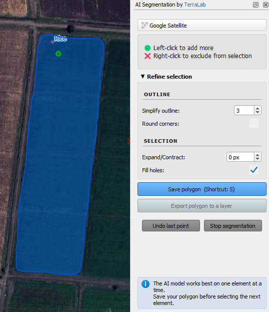
The Sentinel 2 image will have coarser pixels. To be on the save side with mixed pixels, we can contract the polygon a bit.
5. Set Expand/Contract to -5 pixels.
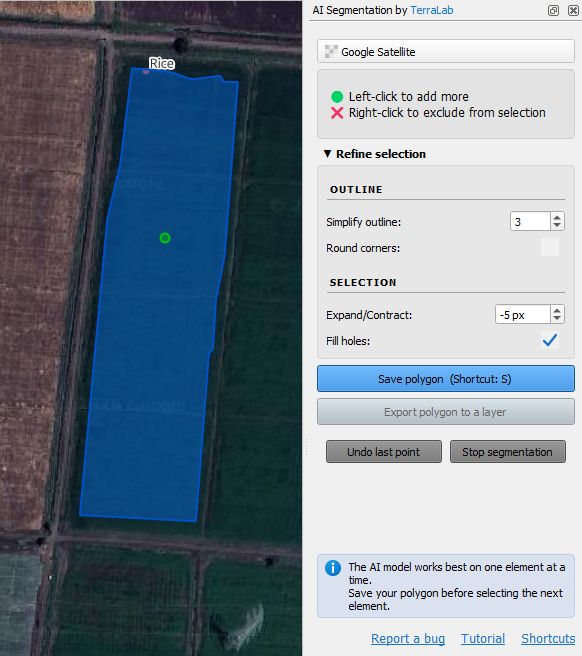
6. Click the blue Save polygon button or type S.
7. Pan to another parcel of the same class (e.g. rice) and repeat the steps. Do this for ~30 parcels of the same class to have a good sample.
Note that you need to pan by dragging the mouse with the scroll button pressed. Panning doesn't work when you click the
button or when you press <space bar> while dragging the mouse. If you use the last two methods, you'll lose the segmented polygons!
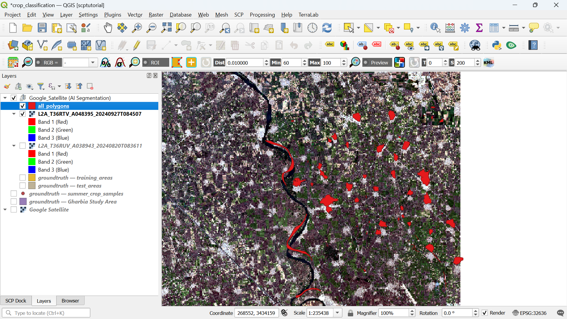
8. Click the green Export 30 polygons to a layer button.
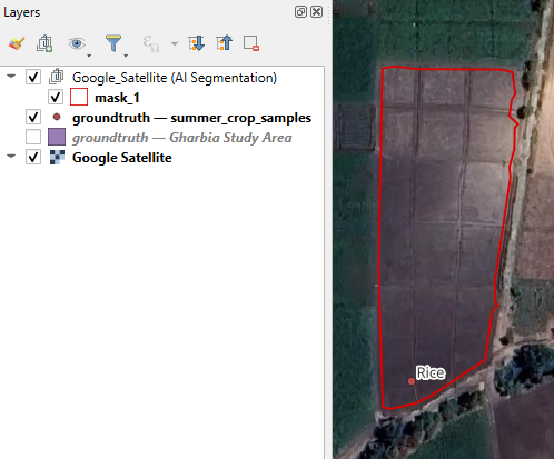
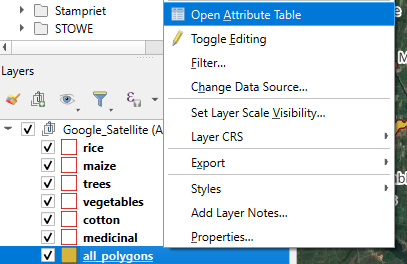
Now you'll find the polygons in a layer under the Google_Satellite (AI Segmentation) layer group in the Layers panel and the segmentation for this class is completed.
9. Click with the right mouse button on the mask_1 layer and choose Rename Layer from the context menu.
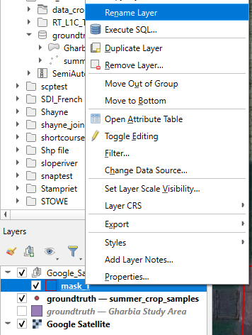
10. Rename it to the name of the class, e.g. rice.
11. Repeat these steps for the other classes. If you can't find 30 polygons, just try as much as you can.
The points are not always clearly in one parcel, so you'll sometimes have to make difficult choices. Also it's not always necessary to delineate the whole parcel if it's very large. The key is to have enough Sentinel 2 pixels in the polygon that can be used for training and testing the classification algorithm.
12. For completeness add also urban and water polygons by identifying them on the satellite image in the same way.
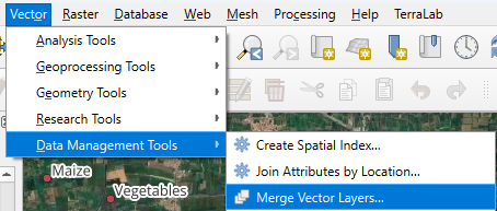
Now we have each class in a separate polygon layer. For our workflow, we need to merge them into one layer.
13. In the main menu, go to Vector | Data Management Tools | Merge Vector Layers....
14. At Input layers, click on  and select the layers to merge. Note that these are only the created polygon layers.
15. Click the arrow to go back to the main dialog.
16. Change the destination CRS to the one of the project, otherwise the polygons will have the projection of the Google Satellite image.
17. Save the result to the geopackage and name the layer all_polygons.
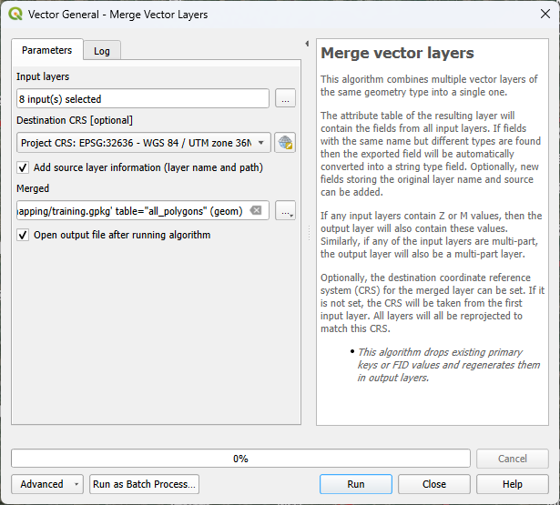
18. Click Run to run the algorithm. Click Close to close the dialog after completion.
19. In the Layers panel, click right on the all_polygons layer and select Open Attribute Table from the context menu.
20. Check the contents of the attribute table.
Here you see that a nice feature of the Merge tool is that it adds the layer name to a field and therefore we have all the classes in a field.
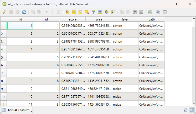
The final task at this stage is to add a column with class ID, which is a unique number for each class.
21. In the attribute table toolbar, click  to toggle to editing mode.
22. Now click on  to open the Field Calculator.
23. In the Field Calculator, type Class_ID at Output field name. Keep Integer (32 bit) as Output field type.
24. Create the expression as in the screenshot below.
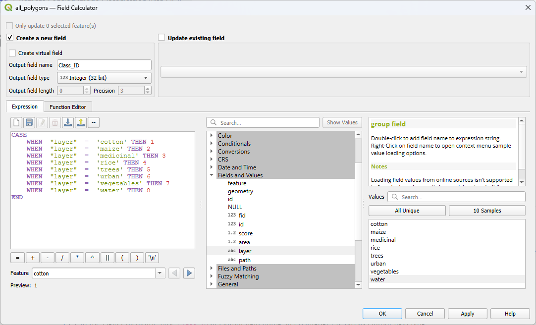
To add field names to the expression, use the middle panel and expand Fields and Values. Then double click on the field that you want to add to the expression, for example layer. It will be added with double quotes. In the right panel, you can view All Unique values in that field. You can add the value to the expression by double clicking on the value, for example water. Values are added with a single quote.
25. Click OK to apply and close the dialog.
26. Check the result. If it's correct, click  to toggle off editing mode and click Save in the popup to save the result.
27. In the Layers panel, remove the individual class polygon layers and the summer_crop_sample layer.
28. Save the project.
In the next section, we'll split the polygons in training and test areas.
4.3. Split Training and Test Areas
To be able to later validate the result of the classification with an error matrix, it's important to not use all polygons in the classification. Therefore, we split the ground truth data in training and test polygons. A typical split is to use 70% for training and 30% for testing. In our case we'll select 70% of the polygons of each class.
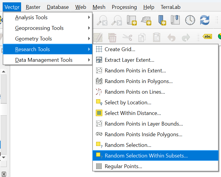
- In the main menu, go to Vector | Research Tools | Random Selection Within Subsets....
- In the Vector Selection dialog, make sure that all_polygons is chosen as the Input layer. For ID field choose Class_ID. Use Percentage of selected features as Method and set the percentage to 70%.
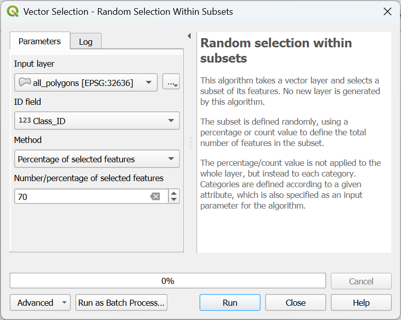
- Click Run to apply the selection. Click Close to close the dialog.
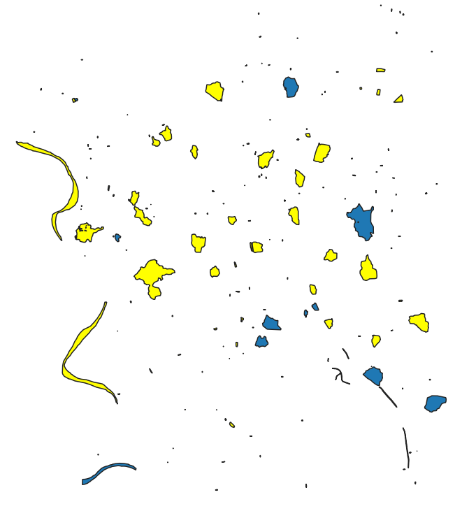
The selected polygons in the all_polygons layer are now highlighted in yellow.
Let's save these polygons in a new layer called training_areas.
4. In the Layers panel, click right on all_polygons and choose Export | Save Selected Features As... from the context menu.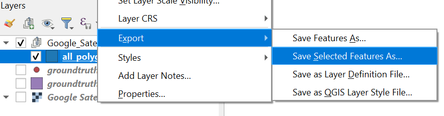
Later, when we use SCP to import training and test areas, we can only load single layer GeoPackages. Therefore, here we'll store the training and test layer in their own GeoPackage, instead of adding them to the existing GeoPackage.
5. In the dialog, use ![]() to browse to the folder where you want to store the layer and use
to browse to the folder where you want to store the layer and use training_areas for both the File name as the Layer name.
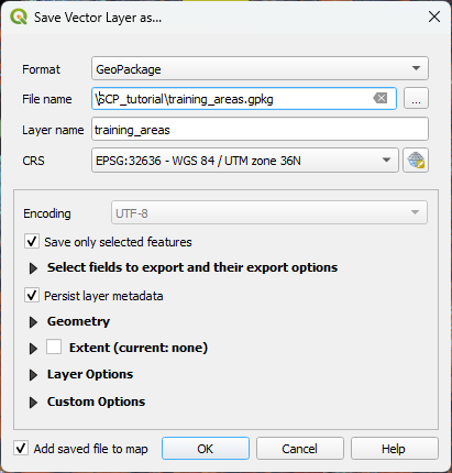
6. Keep the rest as default and click OK to export the layer.
Now we need to export the remaining 30% test areas.
7. Make sure that the all_polygons layer is selected in the Layers panel. In the toolbar, click on the arrow at the right of ![]() and choose Invert Feature Selection.
and choose Invert Feature Selection.
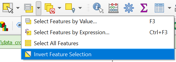
8. Export the selection in the same way as in steps 4 - 6, but name the output GeoPackage and layer test_areas.
Now we have our ground truth dataset ready and can proceed with the remote sensing workflow.
5. Using the Semi-Automatic Classification Plugin
Now we're ready for a workflow with the Semi-Automatic Classification Plugin:
- Download a suitable Sentinel 2 image
- Create a band set
- Import the training data
- Apply the random forest classification algorithm
- Assess the accuracy of the classification
5.1. Install the SCP Plugin
Let's first install the Semi-Automatic Classification (SCP) plugin. You can try to use the official installation instructions from the plugin documentation. If that doesn't work, you can use an experimental version of the plugin with a one-click installer developed by TerraLab, the developers of the AI Segmentation by TerraLab plugin. You can find the installation instructions below.
Note that the alternative SCP plugin with the one-click installer is experimental and comes at your own risk.
- Download the zip file here or from the main course page.
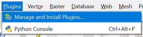
- In the main menu, go to Plugins | Manage and Install Plugins....
- In the dialog, click the
 tab.
tab. - Click
 to browse to the downloaded zip file.
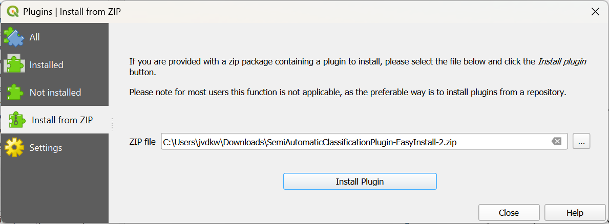
- Click Install Plugin.
- Click Yes in the popup that appears.
- Wait until the message appears that the plugin has been installed and click Close to close the dialog.
- In the dialog that you find behind the one you have closed, click Install Dependencies.
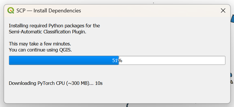
- Wait until the message that the installation is completed and click OK.
- Restart QGIS (save your project if you haven't done that yet).
After restarting you'll find new panels and icons of the SCP plugin, which turns your QGIS in remote sensing software!
You can rearrange the panels a bit so they are in tabs on left side of the QGIS window.
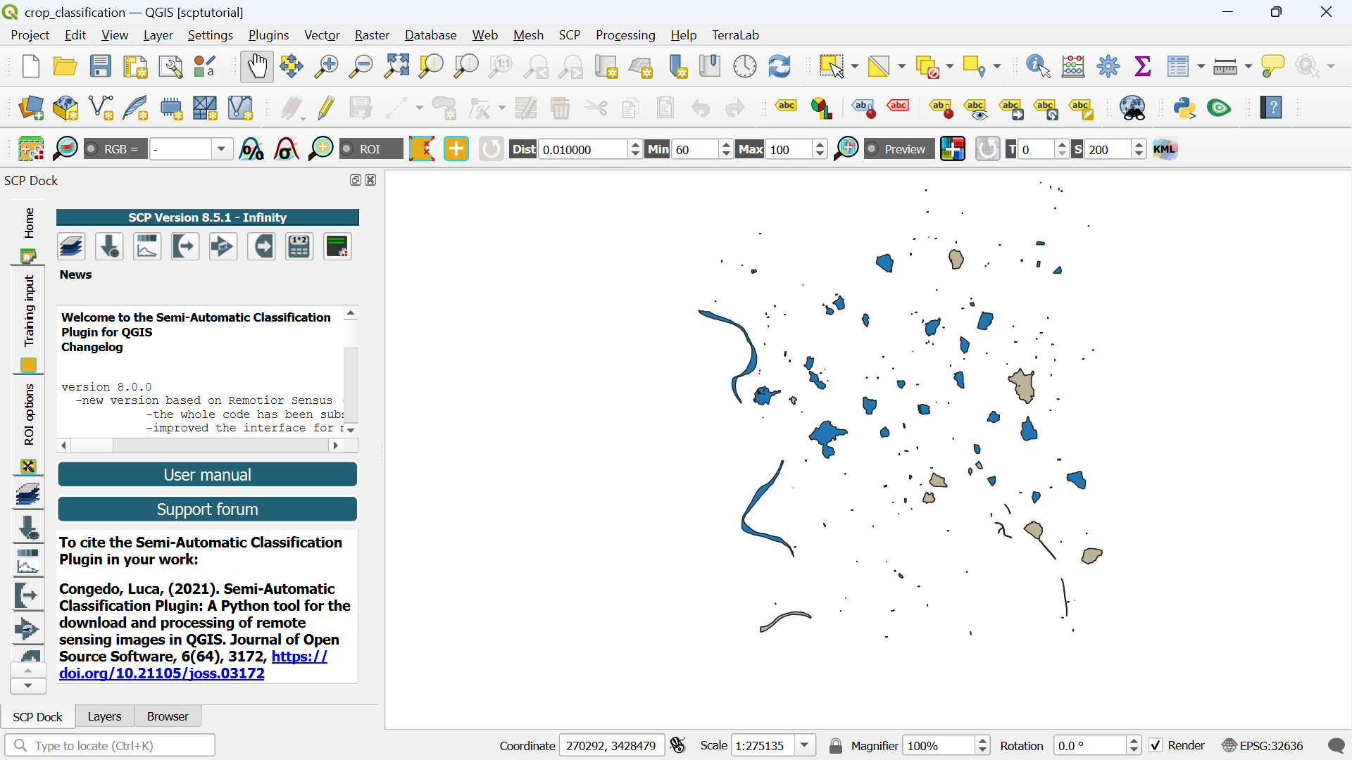
In the next section, we'll download a Sentinel 2 image that we're going to classify.
5.2. Download a Sentinel 2 Image
With the SCP plugin we can easily download Sentinel 2 images.
- In the SCP Dock, click
 to go to the dialog for downloading satellite images.
There are different ways to go to the same dialog. You can click
in the SCP toolbar to open the main SCP dialog. From there you can choose the Download products tab. Another way is to go to the main menu and choose SCP | Download products.
SCP allows you to download the following products:
- Sentinel-2
- Landsat_MPC
- Sentinel-2_MPC
- Landsat_HLS
- Sentinel-2_HLS
- MODIS_09Q1_MPC
- MODIS_11A2_MPC
- ASTER_MPC
- Copernicus_DEM_30_MPC
HLS stands for Harmonized Landsat and Sentinel‑2.
This is a NASA product family that:
- Harmonizes Landsat 8/9 and Sentinel‑2 surface reflectance
- Applies consistent atmospheric correction
- Aligns spectral bands
- Resamples to a common grid (typically 30 m)
- Makes the two missions interoperable for time‑series analysis
SCP can download these directly, which is useful for multi‑sensor classification or temporal analysis.
MPC stands for Mission Performance Centre.
In the context of SCP, MPC products are datasets distributed through the ESA Mission Performance Centres, which provide:
- Pre‑processed, analysis‑ready versions of satellite data
- Consistent metadata
- Standardized formats
- Quality‑controlled products for scientific use
These are typically Level‑2 or analysis‑ready datasets, depending on the mission.
We will use the Sentinel-2_MPC product for our crop type classification.
First we need to select the extent in the Search parameters.
2. In the dialog under Search parameters, click the ![]() icon.
icon.
3. In the map canvas, click with the left mouse button in the upper left corner of the extent you want to use. Click with the right mouse button in the lower right corner of the extent you want to use.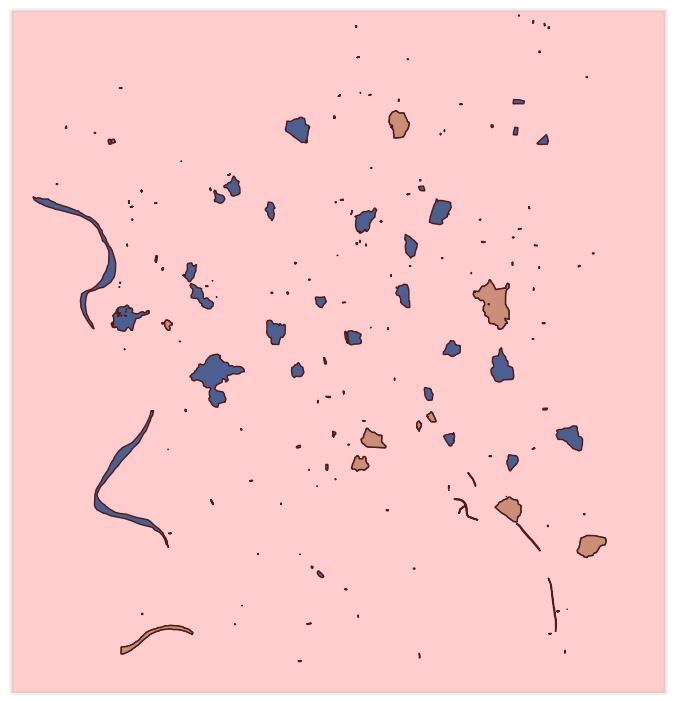
You can further adjust it with the same mouse buttons.
Back in the dialog you will see that the coordinates have been filled in using the Geographic Coordinate System.

Now we can select the data product.
4. Use the drop-down menu at Products to choose Sentinel-2_MPC.
We need to limit our search to the season for which the ground truth was collected.
5. Set the date range to 1 May 2024 - 30 September 2024 and use a Max cloud cover of 20%.
Before we can search for images, we need to give our login details.
6. In the dialog, go to the Login data tab.
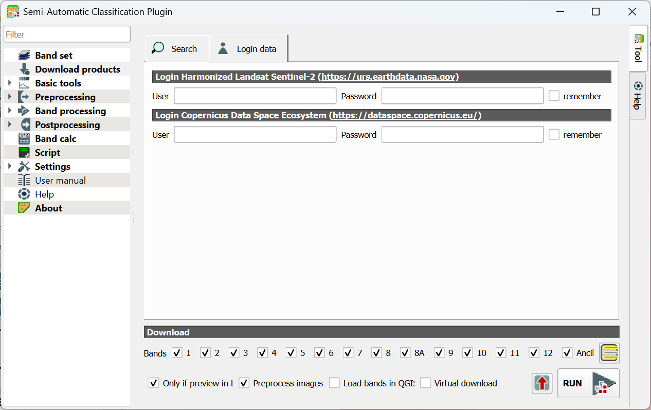
7. Type your credentials or if you don't have an account yet, click the link to create one. Also check the box to remember your account details.
Now we can search the images.
8. Go back to the Search tab and click the Find ![]() icon.
icon.
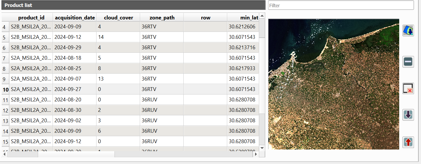
The dialog will return max 20 images in the Product list table. The table shows useful info such as acquisition date and cloud cover.
Let's check the images with 0% cloud cover first.
9. Click on the row of an image with 0% cloud cover and a preview will load in the panel on the right side.
If you found a clear image you can add the preview to the map canvas to check if the extent covers our ground truth data.
10. Click on ![]() to add the preview to the map canvas. Repeat this until you have found an image that covers well our ground truth data.
to add the preview to the map canvas. Repeat this until you have found an image that covers well our ground truth data.
We can also choose which bands we want to download.
For a balanced, high‑performance classification, use:
10 m bands:
- B2 (Blue)
- B3 (Green)
- B4 (Red)
- B8 (NIR)
20 m bands (resampled to 10 m by SCP or QGIS):
- B5, B6, B7 (Red‑edge)
- B8A (Narrow NIR)
- B11, B12 (SWIR)
This gives you 10 bands, which is ideal for crop mapping without overwhelming the classifier.
11. At the bottom of the dialog choose bands 2, 3, 4, 5, 6, 7, 8, 8A, 11 and 12.
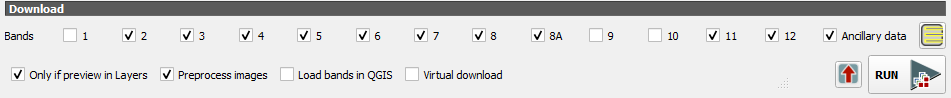
12. Keep the Only if preview in Layers and Preprocess images checked and make sure the other boxes are unchecked.
The Only if preview in Layers setting checks if you have loaded a preview in your map canvas. Only those images will be downloaded. For this exercise make sure you have only one preview image in your project.
Although the MPC is preprocessed, we still need to check the Preprocess images box, otherwise the reflectance values are not scaled correctly.
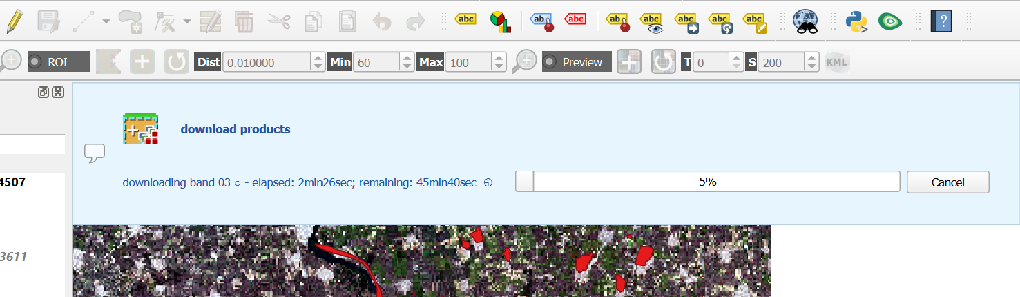
13. Click Run to download the bands. Select the folder where you want to store the files and wait until the download has been completed.
You can see the status of downloading and processing in the main QGIS window.
If your study area is on multiple image tiles, you need to mosaic (merge) them prior to classification. SCP provides a tool for this (out of scope for this tutorial).
If the wifi in the classroom is not working well for downloading the image, please ask the lecturer for the data on a USB stick.
Watch this video for an overview of downloading products with SCP:
After downloading the image, we can proceed with creating the band set.
5.3. Create Band Set
In the previous section, we have downloaded the Sentinel-2 bands as separate GeoTIFF files. For remote sensing, it is however important to consider all bands as a single multispectral image. For this purpose we need to create a band set. A band set is a collection of raster bands that you group together so the Semi‑Automatic Classification Plugin (SCP) can treat them as a single multispectral image. Think of a band set as a virtual satellite image you assemble inside QGIS.
SCP needs to know which bands belong together so it can:
- Compute vegetation indices (NDVI, EVI, etc.)
- Run supervised classification
- Perform PCA, band math, and spectral signatures
- Resample 20 m bands to 10 m if needed
- Keep the correct band order for machine learning
A band set is simply the list of bands you want SCP to use, in the order you choose. A band set stores:
- The file paths to each band
- The band order (important for classification)
- The spatial resolution (SCP can resample automatically)
- Optional cloud masks
- Optional band names or aliases
It does not duplicate data, it just references the rasters you already downloaded.
Let's create our band set.
- Choose the Band set tab. We assume that you were still in the dialog at the Download products tab.
You can see that the band set has been automatically defined as Active band set 2.
If you're not seeing this, you can add the individual bands to the band set by clicking
. In this way you can add already downloaded bands to a band set.
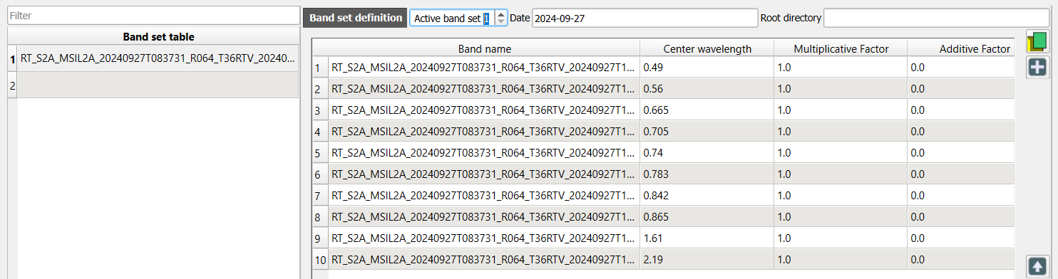
In our case the center wavelengths, units and year are automatically applied to the band set. If this is not the case we can add the center wavelengths and the acquisition date manually to the band set. Under Band quick settings, use the drop-down menu at Wavelength to choose Sentinel-2. At Wavelength unit choose µm and change the Date to the date of the downloaded image, for example 27 September 2024. You can now see that the Band set definition is automatically updated.
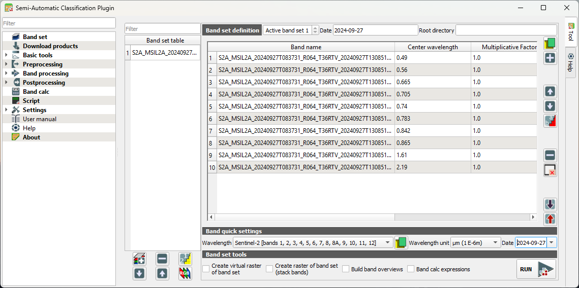
2. Under Band set tools, leave everything unchecked.
Note that our band set is automatically assigned to Active band set 2. Let's make it band set 1.
3. In the Band set table, select the band set that we've just created.
4. Click  to move the band set to the first position.
5. Under Band set definition use the arrows to select Active band set 1.
6. Click  to display the composite in the map canvas.
You can now visualise band combinations from the band set.
9. In the SCP toolbar, you can use the drop down menu to choose a band combination or type the bands with dashes in between.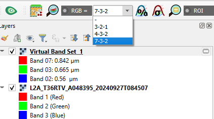
📝 Visualise some composites and try to interpret the results.
Watch this video for more details about band sets in SCP:
Now our remote sensing image is ready and we can proceed with defining the training areas.
5.4. Clip to Study Area
The study area covers only a part of the downloaded Sentinel-2 image. If you use the full image, calculation times will be very large. SCP provides a tool to clip (subset) the satellite image.
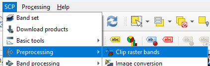
- In the main menu, go to SCP | Preprocessing | Clip raster bands.
- Click to select the boundary coordinates in the map canvas as you did before.
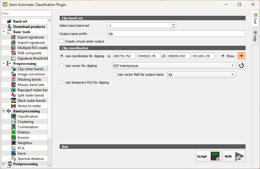
- Click RUN.
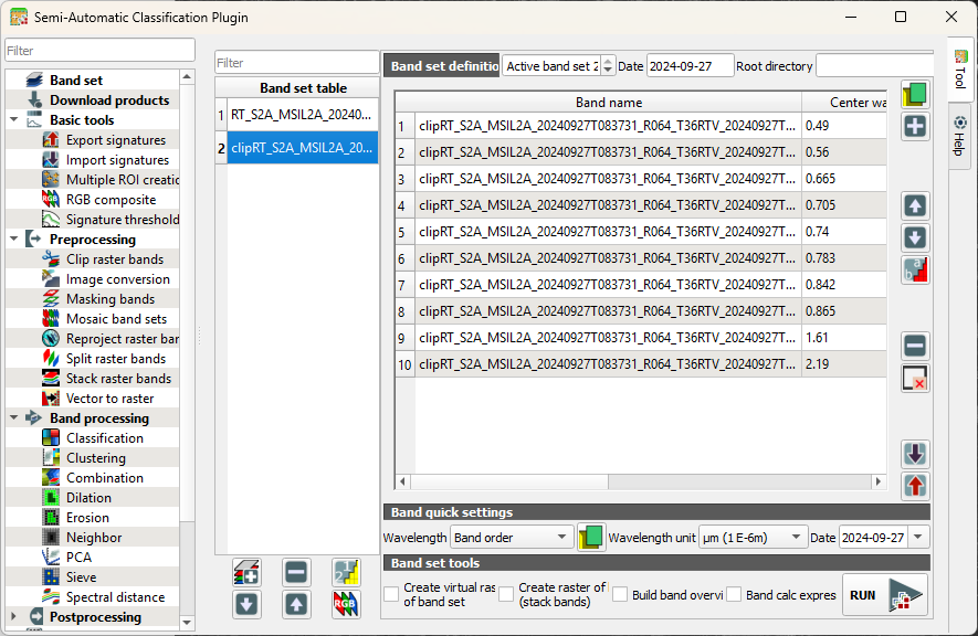
Now we have to create a new band set for the smaller area.
4. Go to the Band set tab and click  to add a new band set or select the empty band set 2 if it's there.
5. Click  to select the files.
6. Under Band quick settings set the Wavelength, Wavelength unit and Date as you did before.
7. Make sure that the Active band set is 2.
8. Click  to load the colour composite.
9. Close the dialog and check the result.
Next, we'll create signatures from the training polygons.
5.5. Import Training Data
The classifier needs training data. With SCP we can easily import the training data polygons from the previous chapter and calculate the spectral signatures for each class.
- Go to the SCP Dock.
- Select the Training Input tab at the left of the dock.
- Click
 to create a new training input.
 - Save the file as training_input.scpx.
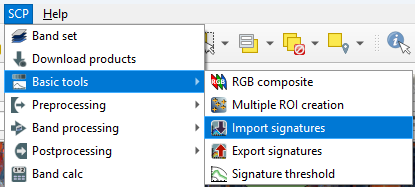
- In the main menu, go to SCP | Basic tools | Import signatures.
- Click on the Import vector section to expand it.
- Click
 to browse to select training_areas.gpkg that we have created in Section 4.3.
SCP uses a two‑level class hierarchy to help you organise training data and produce cleaner, more interpretable land‑cover maps. Macro Classes are the high‑level, thematic categories. Think of them as the main land‑cover groups, such as:
- Vegetation
- Water
- Built‑up
- Bare soil
- Crops
They help you structure your classification and group related detailed classes together.
Micro Classes are the detailed, fine‑grained categories inside each macro class. Examples:
Macro Class Micro Classes Vegetation Forest, Grassland, Shrubland Water River, Lake, Irrigation Canal Crops Wheat, Maize, Rice, Sugarcane When you create training areas in SCP:
Each area is assigned a Micro Class ID.
Each Micro Class belongs to a Macro Class ID.
During classification:
The classifier predicts Micro Classes.
You can later aggregate them into Macro Classes for simpler maps or reporting.
In this tutorial we don't use this hierarchy. Therefore we define the same fields for both micro and macro classes.
8. Select the fields as in the screenshot below. Remember that the layer field contains the class names.
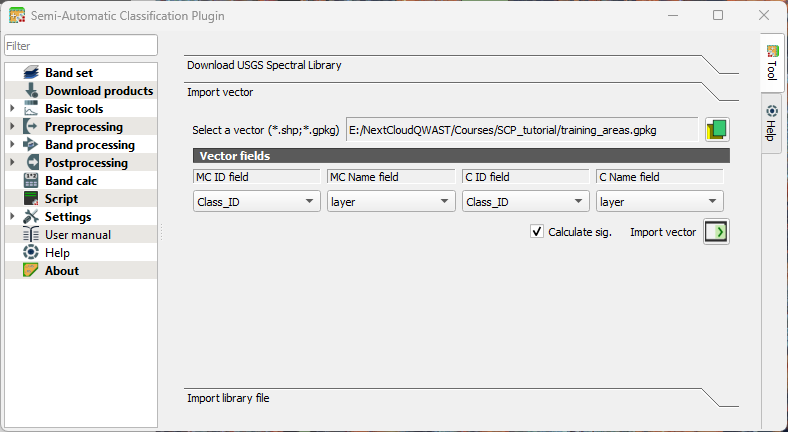
9. Keep the rest as is and click Import vector  .
.
Wait until the process has finished. This can take a while.
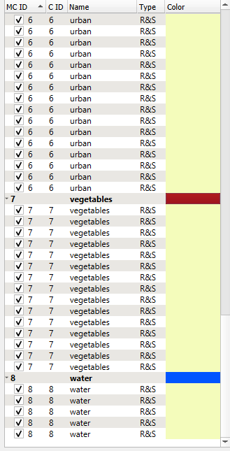
Let's add the class colours to the training areas. Training areas are also called Regions of Interest (ROI).
10. Click on the Color column to change the colour of a Macro Class (the bold line in the table). We don't need to change this for the micro classes.
5.6. Evaluate Training Areas
We can compare spectral signatures of the ROIs. Let's first compare signatures of one class to check the inter class variability.
1. Select all cotton signatures by selecting the row that only mentions cotton. Then click  to add their signatures to the spectral signature plot.
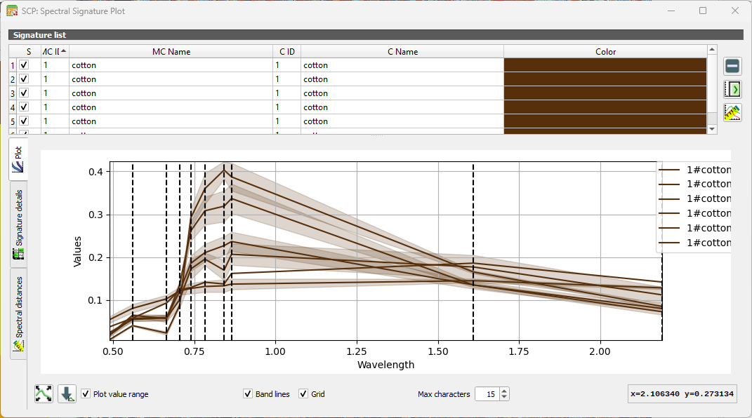
You can show/hide specific curves by checking/unchecking the box in the first column of the table. The vertical dashed lines show the bands.
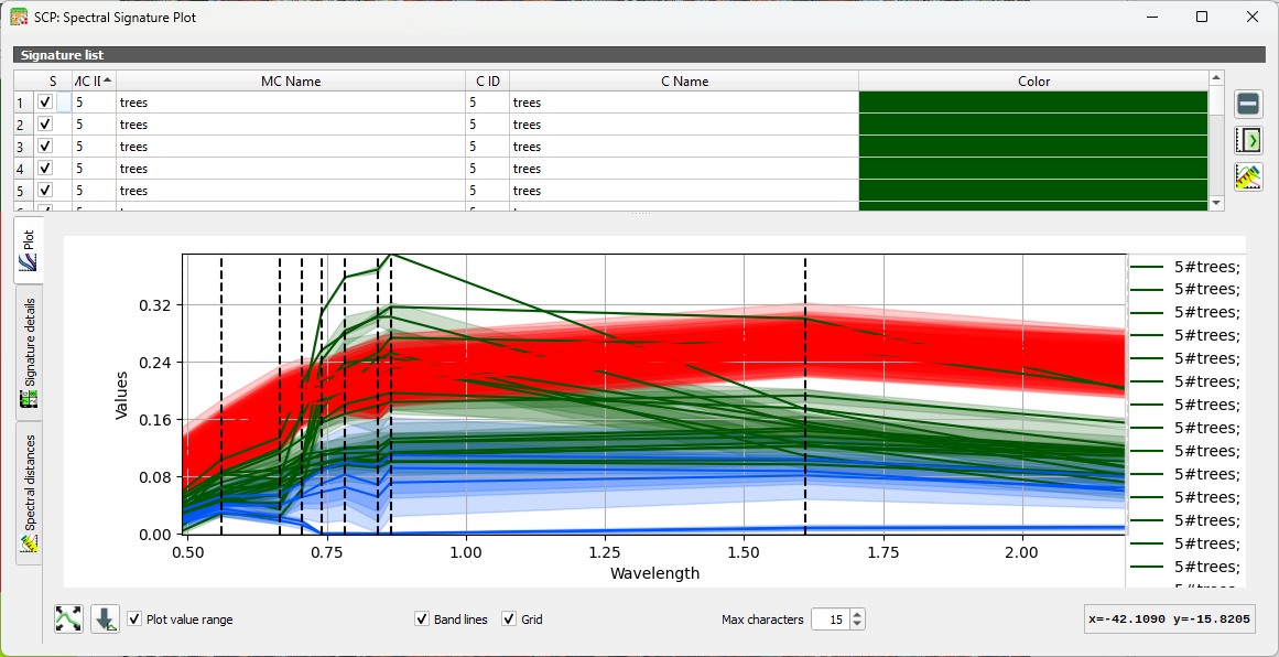
2. Repeat this for several classes. You can add and remove signatures from the table in the Spectral Signature Plot dialog.
3. Now compare signatures of different classes.
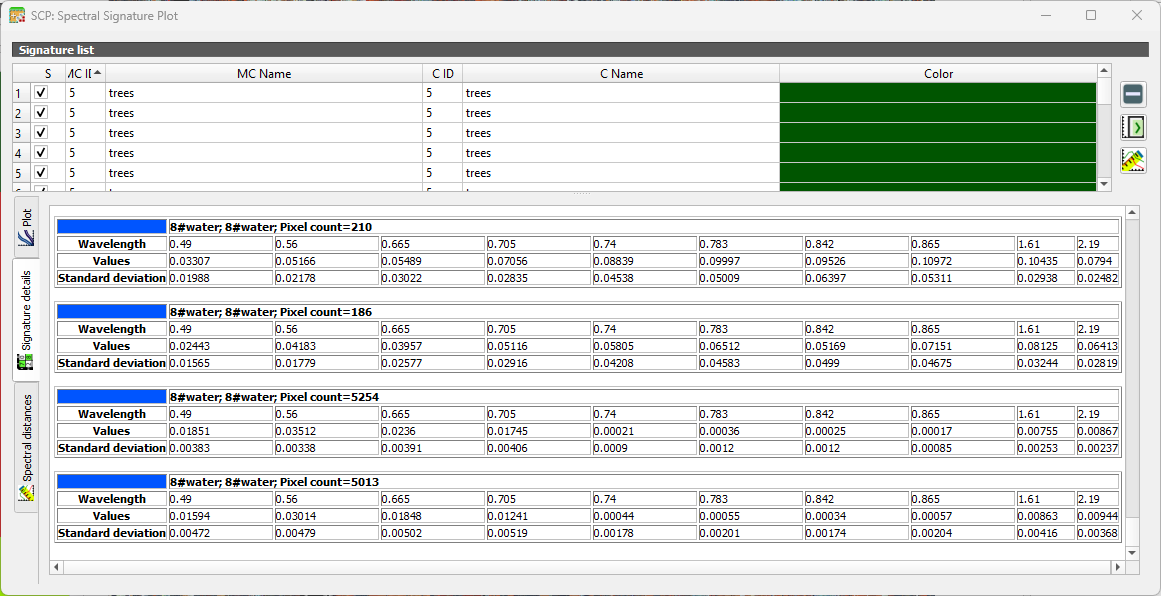
Under the Signature details tab you can see statistics for each ROI.
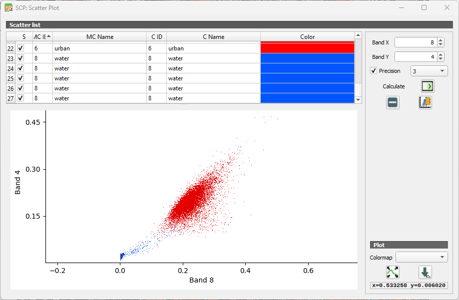
Another way to look at the classes is in the Feature Space Plot. The Feature Space Plot is a visual tool that helps you understand how different land‑cover classes are distributed in spectral space. It’s especially useful before classification, because it shows whether your classes are spectrally separable, a key requirement for good supervised classification.
A Feature Space Plot displays:
- Two spectral bands on the axes (e.g., Band 4 vs Band 8)
- Training samples (ROIs) plotted as points
- Colors representing different classes
- Clusters showing how similar or different classes are in spectral space
You can think of it as a scatterplot of reflectance values. If two classes form distinct clusters, the classifier can easily tell them apart.
If clusters overlap heavily, the classes may be confused during classification. This often happens with:
- Similar vegetation types
- Bare soil vs built‑up
- Water shadows vs deep water
Points far away from the main cluster may indicate:
- Mislabelled training samples
- Mixed pixels
- Cloud shadows or noise
 .
.
5.7. Setup the Random Forest Classifier
Random Forest is one of the most versatile and widely used machine‑learning algorithms for remote sensing. Instead of relying on a single decision tree, a Random Forest builds many trees, each trained on a slightly different subset of the data, and then lets them “vote” on the final class. This ensemble approach makes the method remarkably robust: it handles noisy training data, reduces overfitting, and performs well even when classes overlap in spectral space.
For remote sensing applications, Random Forest is especially attractive because:
- It works well with high‑dimensional data, such as multispectral or hyperspectral imagery.
- It can model complex, non‑linear relationships between spectral bands and land‑cover classes.
- It provides measures of variable importance, helping you understand which bands or indices contribute most to the classification.
- It requires minimal parameter tuning, making it accessible for beginners while still powerful for advanced users.
More info can be found here.
Let's configure the Random Forest classifier in SCP.
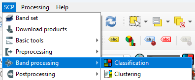
- In the main menu, go to SCP | Band processing | Classification.
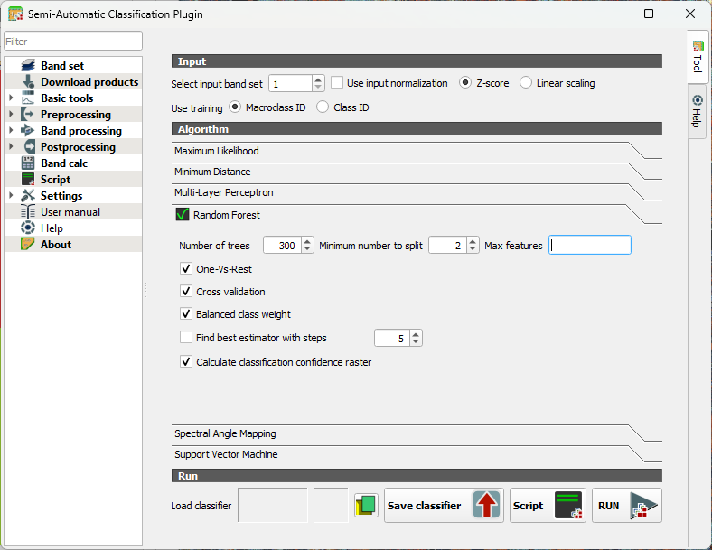
- Under the Algorithm section click on Random Forest to expand the configuration settings.
You’ll see several parameters you can adjust. Each one influences how the forest of decision trees is built and how your final land‑cover map is produced.
Number of Trees
- Defines how many decision trees the algorithm will grow.
- More trees generally improve stability and accuracy because the “forest” can average out noisy or biased trees.
- Typical values range from 100 to 500, but SCP allows you to go higher if needed.
Minimum number to split
- Sets the minimum number of samples required to create a new split or leaf.
- Higher values make trees more conservative and reduce overfitting.
- Lower values allow more detailed splits but may capture noise.
Max features (per split)
- Determines how many predictor variables (bands, indices, etc.) each tree considers when splitting nodes.
- Randomizing this selection is what gives Random Forest its strength.
When you run a Random Forest classification in SCP, you’ll see a few extra options that help the algorithm deal with tricky situations. One‑Vs‑Rest tells the classifier to look at each class separately: it learns to distinguish one class from all the others, which can help when some classes are harder to separate.
Cross validation is a built‑in way for SCP to check how well your model is likely to perform on new data. It repeatedly trains and tests the classifier on different subsets of your samples, giving you a more reliable accuracy estimate without needing a separate validation set.
If your training data is unbalanced, for example, if you have many samples for vegetation but only a few for water, you can turn on Balanced class weight. This gives smaller classes more influence during training so they aren’t overshadowed by the larger ones.
SCP can also find the best estimator for you. This means it automatically tries different combinations of Random Forest settings and picks the one that performs best. It’s a helpful shortcut when you’re not sure which parameters to choose.
Finally, you can create a classification confidence raster, which shows how confident the model is about each pixel. High values mean the trees in the forest strongly agreed on the class; lower values highlight areas where the model was uncertain. It’s a great way to visualize where your map is most reliable and where you might want to be cautious.
Let's configure some settings for our first try.
3. Keep the number of trees as default so the preview in the next section will calculate fast. After that we'll increase the value. 300-500 is typically used.
4. Toggle on One-Vs-Rest. This helps separate similar crops by giving each class its own focused model. It reduces confusion when spectral signatures overlap.
5. Toggle on Cross validation. This will give us an internal accuracy estimate.
6. Toggle on Balanced class weight. In our case some classes have many more training samples than others. It ensures that minority classes aren't ignored.
7. Toggle on Calculate classification confidence raster. In this way we can identify ambiguous pixels.
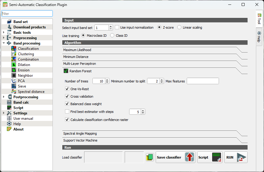
8. Close the dialog.
Now we've configured the classifier, we can apply it to our image in the next section.
5.8. Preview the Classification
A nice feature of SCP is that we can preview the classification for a small area.
- In the SCP toolbar, click
 to activate the classification preview pointer.
 - Click somewhere in the image.
SCP will now calculate the preview classification. That will take a couple of minutes for the first one. The next ones will be calculated faster.
3. Click at several locations to see the preview.
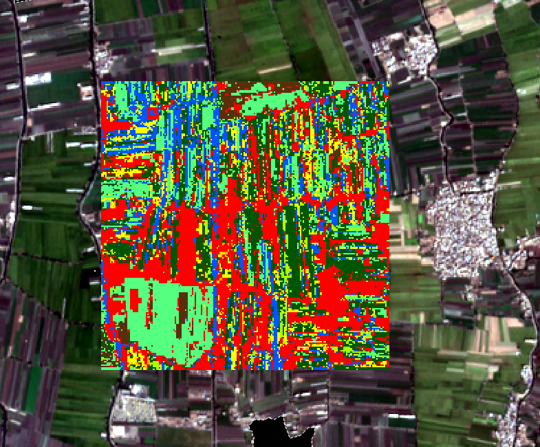
In the next section, we'll classify the entire image.
5.9. Classifiy the Entire Image
Before we'll classify the entire image, we'll first increase the number of trees.
- In the main menu, go back to SCP | Band processing | Classifcation.

- Set the number of trees to 300.
- Click RUN.
- Browse to the location where you want to save the output GeoTIFF and save it as cropmap.tif.
This will take a while (2 hours on my pc).
This video shows an overview of the Random Forest Classification in SCP:
In the next section we'll evaluate the result.
5.10. Accuracy Assessment
Once a land‑cover map has been produced, the next essential step is to evaluate how well the classification represents reality. This is where accuracy assessment comes in. In the Semi‑Automatic Classification Plugin (SCP), accuracy assessment provides a structured way to compare your classified map with reference data and quantify how reliable your results are.
In this chapter, you’ll learn how SCP uses your test areas to build an error matrix, calculate key metrics such as overall accuracy, producer’s and user’s accuracy, and the Kappa coefficient, and help you understand where the model performs well and where it struggles. Rather than treating classification as a “black box,” accuracy assessment encourages you to look critically at the outcomes, identify common sources of confusion, and reflect on how training data, class definitions, or spectral similarity influence the final map.
Let's use the SCP tools for accuracy assessment.
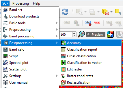
- In the main menu go to SCP | Postprocessing | Accuracy.
- Under Input, choose the cropmap as the classification to assess and select test_areas that we have created before as the reference vector. Use the
 button to refresh the layers list in the drop-down menu. At Vector field choose Class_ID.
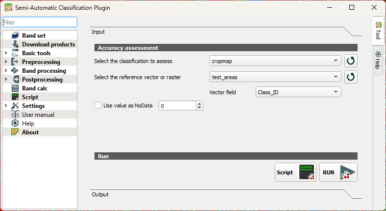
- Click RUN.
- Choose an output location and filename for the rasterized test areas.
When the accuracy assessment is done, the tool will show you the results in the Output section of the dialog.
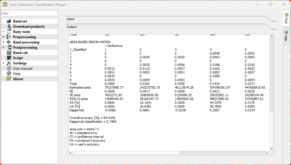
Interpret the result with the following statistics that were calculated:
Standard Error
Shows how much uncertainty there is in an accuracy estimate. Smaller values mean the estimate is more stable and would change little if you repeated the assessment.
Confidence Interval
Gives a range in which the “true” accuracy is likely to fall. Example: 85% ± 3% means the real accuracy is probably between 82% and 88%.
Producer’s Accuracy
Indicates how well the classifier avoided omitting a class. Interpretation: Of all real pixels of this class, how many were correctly mapped? Low values mean many pixels of that class were missed.
User’s Accuracy
Indicates how reliable the map is for someone using it. Interpretation: When the map labels a pixel as this class, how often is that correct? Low values mean many pixels were incorrectly assigned to that class.
Overall Accuracy
The percentage of all validation samples that were correctly classified. A simple, general measure of performance.
Kappa Coefficient
Compares your classification to what would be expected by random chance. Values near 1 indicate strong agreement; values near 0 mean the map is not much better than guessing.
5.11. Conclusion
In this tutorial, you walked through the complete workflow for preparing and classifying remote‑sensing imagery in QGIS. You created a clean working environment, prepared ground‑truth data, segmented parcels using the AI Segmentation plugin, and applied the Semi‑Automatic Classification Plugin to build and evaluate a Random Forest model. Together, these steps showed how traditional GIS methods and modern AI‑assisted tools can complement each other to produce accurate, reproducible land‑cover maps.
By now, you should feel confident in setting up a classification project, organizing training data, running supervised classification, and assessing the quality of your results. These skills form the foundation for more advanced remote‑sensing analyses, whether you are mapping crop types, monitoring land‑use change, or supporting water‑productivity assessments.