Tutorial: Stream and Catchment Delineation
| Site: | OpenCourseWare for GIS |
| Course: | Hydrological Analysis in QGIS - QGISUC2026 |
| Book: | Tutorial: Stream and Catchment Delineation |
| Printed by: | Guest user |
| Date: | Friday, 2 October 2026, 3:00 AM |
Description
Table of contents
- 1. Introduction
- 2. Theory
- 3. Download DEM
- 4. Reproject DEM
- 5. Create a Subset of the DEM
- 6. Fill Sinks and Calculate Flow Direction
- 7. Styling Flow Direction
- 8. Delineate Streams
- 9. Delineate the Catchment
- 10. Clipping layers to the catchment boundary
- 11. Styling the Resulting Catchment Area
- 12. Storing the Data in a GeoPackage
- 13. Conclusions
1. Introduction
One of the most important uses of GIS in hydrology is the delineation of catchments and streams. This lesson presents a generic workflow for stream and catchment delineation for areas where only open data is available. The Shuttle Radar Topography Mission (SRTM) 1 Arc Second DEM will be used. The workflow will be applied to the Rur catchment in Germany.
We will use the native QGIS tools for hydrology that are available from QGIS 4.4.
After this lesson you will be able to:
- find and download SRTM DEM
- reproject rasters
- create subsets of rasters
- fill sinks in a DEM
- calculate and style flow direction raster layers
- calculate Strahler orders
- delineate streams
- delineate catchments
- style layers for visualising catchments
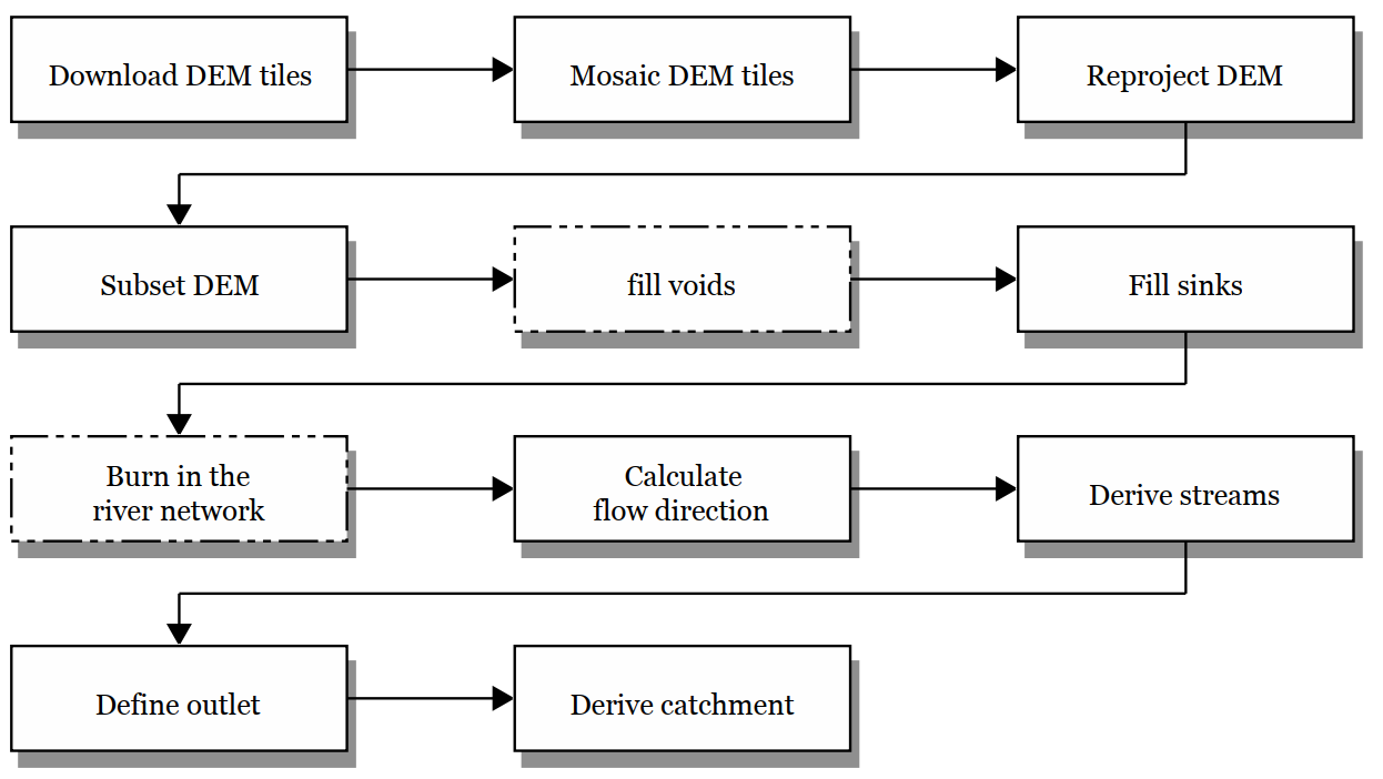
In order to delineate a catchment from a DEM in GIS we need to follow these steps (details covered in this lesson):
1. Download the DEM tiles of your study area. Make sure that the tiles cover at least the study area and that the catchment you want to derive is covered completely. Better to take it a bit larger to avoid boundary effects.
2. If your study area is covered by multiple DEM tiles, you need to mosaic (merge) the tiles to create a single raster DEM layer.
3. The DEM tiles might be in a different coordinate system then desired. In that case you have to reproject the DEM layer to the projection you want to use in the study area.
4. In the case that the merged tiles are much larger than your study area, you can subset (clip) it to a smaller area to reduce calculation time.
5. Interpolate voids when pixels with no data exist in the DEM.
6. Make a hydrologically correct DEM by filling sinks and removing spikes.
7. Calculate the flow direction for each cell.
8. Derive the drainage network.
9. Calculate the catchment for the outflow point of the catchment.
When a map with the stream network already exists, the procedure can be improved by "burning" the river network into the DEM. In that way the DEM is always lower at rivers and runoff will follow the actual river network. This is beyond the scope of this chapter.
The matrials for this lesson can be downloaded from the main lesson page. The next section covers how to download the SRTM tiles from USGS EarthExplorer. These are also included in the course data.
2. Theory
2.1. Digital Elevation Models in GIS
Watch this video on Digital Elevation Models in GIS.
2.2. Stream and Catchment Delineation
Watch this video on the theory of stream and catchment delineation.
3. Download DEM
For the Rur study area, we will download the tiles from the SRTM 1 Arc-Second global data set. Since the end of 2014 a 1-arc second global digital elevation model (approximately 30 meters at the equator) has been released as open data. Most parts of the
world have been covered by this dataset ranging from 54 degrees south to 60 degrees north latitude. A description of the SRTM data products can be found here.
The following steps explain
how to download the SRTM DEM tiles for the study area using the OpenTopography DEM Downloader plugin. With the plugin you can download DEMs from OpenTopography.org for a user-selected extent.
1. Start QGIS Desktop. We’ll start with a new project. In the Browser panel, add the folder with the data for this lesson to the Favorites as you learned in the previous lesson.
2. Drag the boundingbox.shp layer from the Browser panel to the map canvas.
This polygon defines the boundary of our initial analysis. Normally you have to create such a polygon yourself or use the map canvas coordinates. We need this to clip the DEM to the study area. Note that the projection of the project (on-the-fly reprojection) is now set to the
projection of the boundingbox layer. You can check it in the lower right corner of the screen.

We will work in this projection during this exercise.
3. Install the OpenTopography DEM Downloader plugin from the Plugins Manager. Go to the main menu and choose Plugins | Manage and Install Plugins....

4. In the Plugins Manager search for OpenTopography and install the plugin.
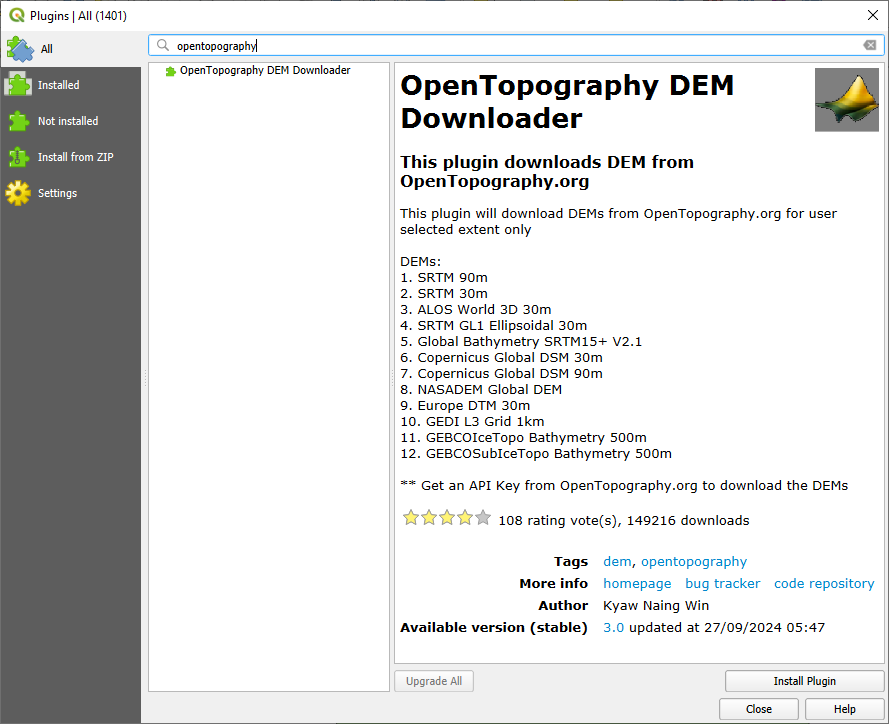
 button in the toolbar.
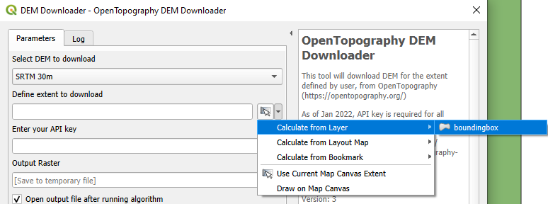
 to copy the API key.
 to browse to a folder where you want to store the data for this project. Remember to stick to the good practice instructions for file and folder names (no spaces, accents, -, etc.). Always use the
  button in QGIS dialogs to choose the output location! Name the file SRTM.tif.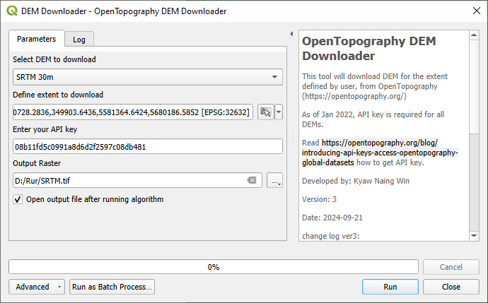
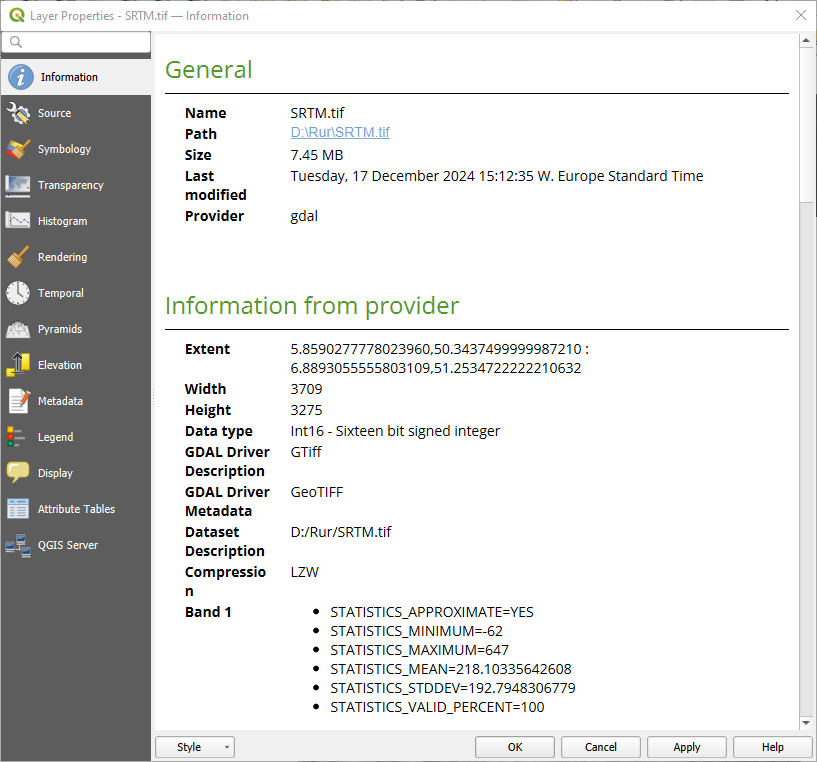
- What is the projection?
- What are the map units?
Watch this video to check the steps:
4. Reproject DEM
The DEM is in its original Lat/Lon Geographic Coordinate System (GCS) with datum WGS 84 (EPSG: 4326). It is not recommended to use a GCS for DEM analysis, because the z units (e.g. meters) are different than the x and y units (degrees). We need to choose
a projection for our project. If the project covers one country we can choose a national projection. In our case, however, the project covers multiple countries (Germany, the Netherlands, and Belgium). Therefore we will use a global projection: UTM
Zone 32 North, with WGS-84 as datum.
We can find the EPSG codes at http://www.spatialreference.org
1. Use the website to search for UTM 32N wgs 84. You can leave
QGIS running and open a browser.
The figure below shows the result.
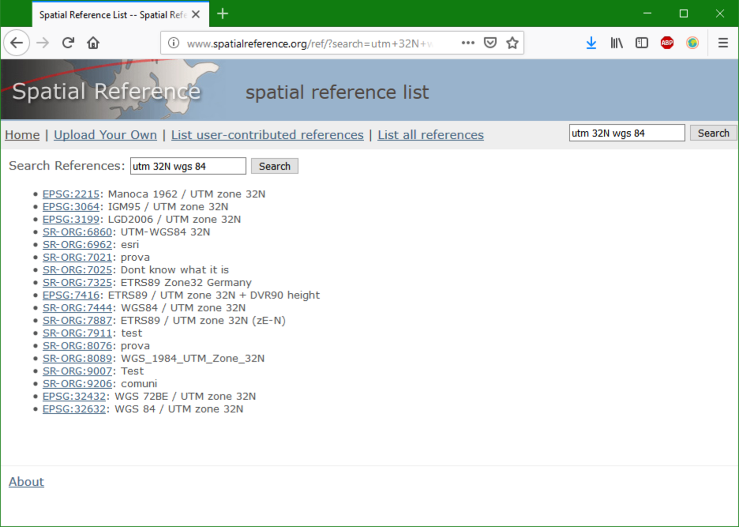
We need to take a look at
the EPSG codes. We will use EPSG: 32632 throughout this project - clicking on it will provide more details. Note that this is the same projection the boundingbox layer has and was used for setting the projection of our project when we loaded
the boundingbox layer as our first layer.
Now we are going to reproject the DEM from unprojected GCS (Lat/Lon WGS 84 - EPSG: 4326) to UTM Zone 32 North / WGS 84 (EPSG: 32632).
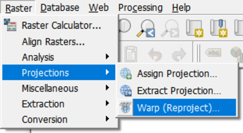
2. From the main menu choose Raster | Projections | Warp (Reproject).
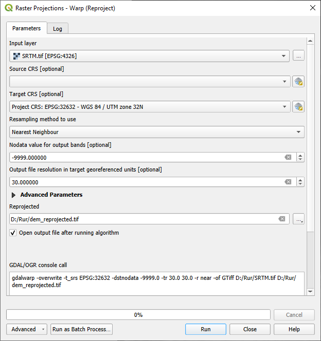
3. In the Warp (reproject) window, choose the Project CRS: EPSG:32632 - WGS 84/UTM zone 32N as Target CRS.
4. Now complete the dialog:
- Make sure the Input layer is SRTM.tif.
- For the Resampling method we choose
Nearest Neighborto preserve the elevation values of the original files. - Set the No data value for output bands to
-9999because when the raster layer is reprojected there will be "no data" at the borders. In this way we define that "no data" has a value -9999 and will not be visualised and treated as "data". - Set the Output file resolution to
30m. - Browse to your exercise folder and name the output file
dem_reprojected.tif. Make sure you choose a GeoTIFF as output format.
The dialog should now look like the figure below.
Note the gdalwarp command that will be executed in the background. Under Advanced Parameters, we could have specified the extent of the output file based on the boundingbox layer. In that way the dem_mosaic layer is reprojected and clipped in one step.
5. Click Run to run the algorithm. After running,
click Close to close the window.
The re-projected DEM now appears in the map canvas.
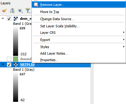
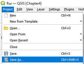
This is a good time to save your project.
7. In the main menu, go to Project | Save as... and browse to the folder where the other data of this exercise is stored. Name the project Rur.
5. Create a Subset of the DEM
In order to reduce the calculation time of the algorithms, we will subset (or clip) the raster layer to the boundingbox polygon.
1. Now, from the main menu select Raster | Extraction | Clip Raster by Mask Layer.
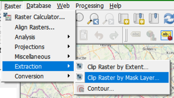
2. In the Clip Raster by Mask Layer dialog, choose dem_reprojected for the Input layer. For Mask Layer, choose boundingbox. Check the box to Keep resolution of input raster and keep the defaults for the other options. Choose dem_subset for the Clipped (mask) output and click Run. Click Close when done.
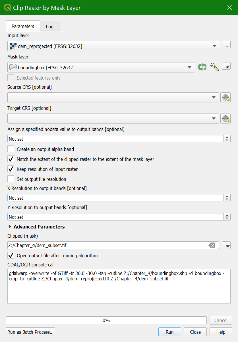
Often you'll not have a bounding box shapefile. In that case you can choose Raster | Extraction | Clip Raster by Extent. Then you can drag a box in the Map Canvas and use that for clipping. While using that, make sure your on-the-fly reprojection is similar to the layer that you want to clip, because the map canvas coordinates are used by the algorithm.
3.
Now you can remove dem_reprojected from the layers list as we have done before for other layers that are no longer needed.
Watch this video to check the steps in this section:
5.1. Styling the DEM
By default, QGIS styles raster layers with the Singleband gray renderer. As you have learned in Lesson 3, the software does not know the raster data type (e.g. boolean, discrete or continuous) and how the user wants to present the information.
To help interpret the results, it is good practice to intuitively style your layers.
The DEM is a continuous raster. Continuous rasters represent gradients and can therefore contain real numbers ((also called decimal numbers or floating point). Continuous rasters are styled in QGIS using ramps from the Singleband pseudocolor renderer in the Layer Styling panel.
1. Select the dem_subset layer and click  to open the Layer Styling panel (or press
 F7).
2. In the Layer Styling panel, choose Singleband pseudocolor from the drop-down
list.
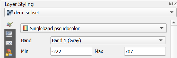
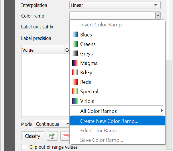
3. Click the arrow at Color ramp and choose
Create New Color Ramp from the dropdown menu.
4. In the popup Color ramp type dialog choose Catalog: cpt-city from the drop-down list.
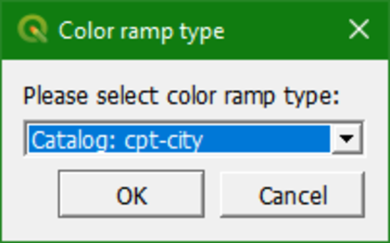
The cpt-city catalog
has a lot of useful preset color ramps.
5. Choose Topography | Elevation. Note that cd-a and sd-a are also nice choices.
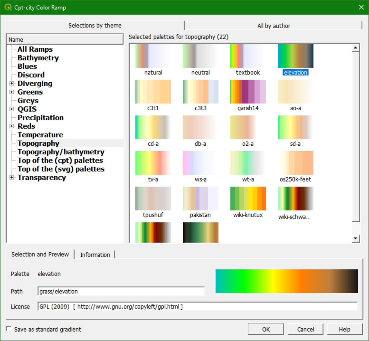
6. Click OK to close the dialog.
This gives us more intuitive colors in the DEM where we can clearly distinguish higher and lower areas (if you don’t see the colors applied, click Classify).

Now we will further improve the vizualisation.
7. Right-click on the dem_subset layer in the Layers panel and select Duplicate Layer.
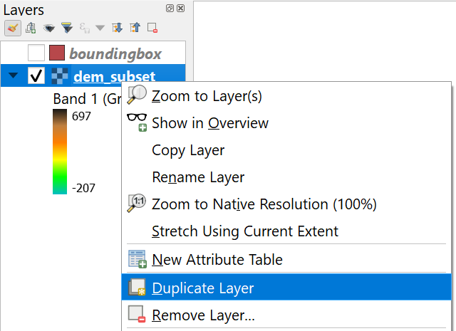
This creates a copy of the dem_subset layer
called dem_subset copy.
8. Uncheck the dem_subset layer, check the dem_subset copy layer and rename it to hillshade: right-click the layer and choose Rename Layer from the context menu.
9. In the Layer Styling panel, which should still be open, make sure that
the hillshade layer is now selected. In the drop-down list change Singleband pseudocolor to Hillshade.
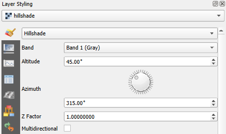
Now the hillshade layer is vizualised with a shading.
- Which direction is the illumination coming from?
- Is this possible in reality?
Hillshade gives the best results with an artificial illumination in the northwest, which in reality can not exist in the Northern Hemisphere. If you move the dial in the Layer Styling panel to the southwest, you will see an inverted relief. Also note that there is a Resampling section. The default resampling method for both Zoomed in and Zoomed out is Nearest Neighbor. This method is fine for categorical data however, elevation is considered continuous data.
10. You should therefore choose a Zoomed in resampling method of Bilinear and a Zoomed out resampling method of Cubic.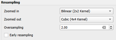
Next, we're going to blend the DEM with the hillshade layer.
11. Switch
on the dem_subset layer by checking the box.
12. In the Layer Styling panel make sure the dem_subset layer is selected. In the Layer Rendering block of the panel, change the Blending mode to Multiply.
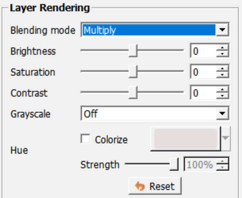
As you can see, blending gives a much nicer
effect than transparency. With transparency the colors will fade. Now we can clearly see the elevation differences: the gradient from south to north and the valleys where we expect the streams.
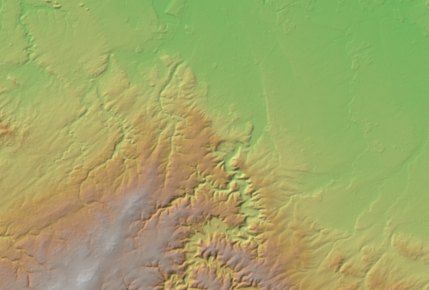
Blending modes allow for more elegant rendering between GIS layers. They can be much more powerful than simply adjusting layer Opacity. Blending modes allow for effects where the full intensity of an underlying layer is still visible through the layer above. There are 13 blending modes available. See here for more info.
Watch this video to check the steps of this section:
6. Fill Sinks and Calculate Flow Direction
Raw, unprocessed DEMs have artifacts such as depressions. Artifacts are a result of the DEM acquisition process and must be removed before a DEM can be used for hydrological analysis, like catchment and stream delineation or hydrological modelling. There are several algorithms for filling sinks. Here we'll use the native Fill Sinks (Wang & Liu) tool. This tool fills the sinks and creates a filled DEM suitable for further hydrological analysis.
- In the Processing Toolbox, go to Raster terrain analysis | Fill sinks (Wang & Liu).
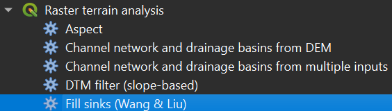
2. In the dialog, choose dem_subset as Input layer. Save the Output layer (filled DEM) as dem_filled.tif and Output layer (flow directions) as flowdirections.tif.
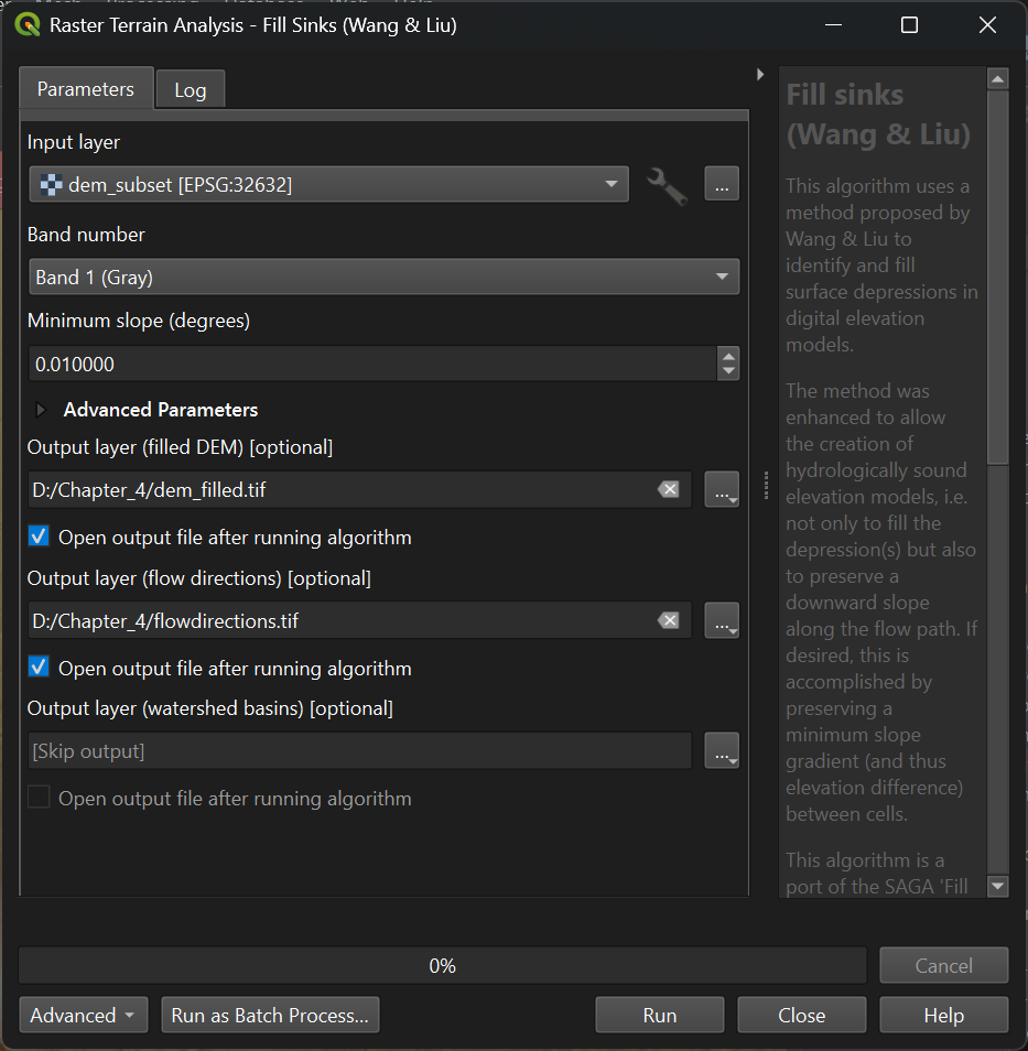
3. Keep the rest as default and click Run. Click Close after processing.
7. Styling Flow Direction
The next step is to fill the sinks (artificial depressions in the DEM) and calculate the flow direction raster. PCRaster does both in one step with the lddcreate tool. Check the documentation for the details.
1. In the Processing Toolbox go to PCRaster | Hydrological and material transport operations | lddcreate
2. In the Lddcreate dialog choose dem as DEM layer. Keep all other defaults so it will fill the sinks completely. Save the results to flowdirection.map.
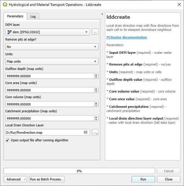
3. Click Run. This can take a few minutes before the result appears in the map canvas. Click Close to close the dialog.
The lddcreate tool fills the sinks in the DEM and results in a local drain direction (flow direction) map. If you need the filled DEM, you can use the lddcreatedem tool.
In the next step we'll style the flow direction map.
7.1. Styling the Flow Direction Layer using Arrows
We can further improve the styling of the flowdirection layer by adding arrows. This can be done using the mesh styling functionality of QGIS. To use that functionality, we need to convert the PCRaster LDD to a mesh format. We can do that with the Crayfish plugin.
1. Install the Crayfish plugin from the Plugins Manager.
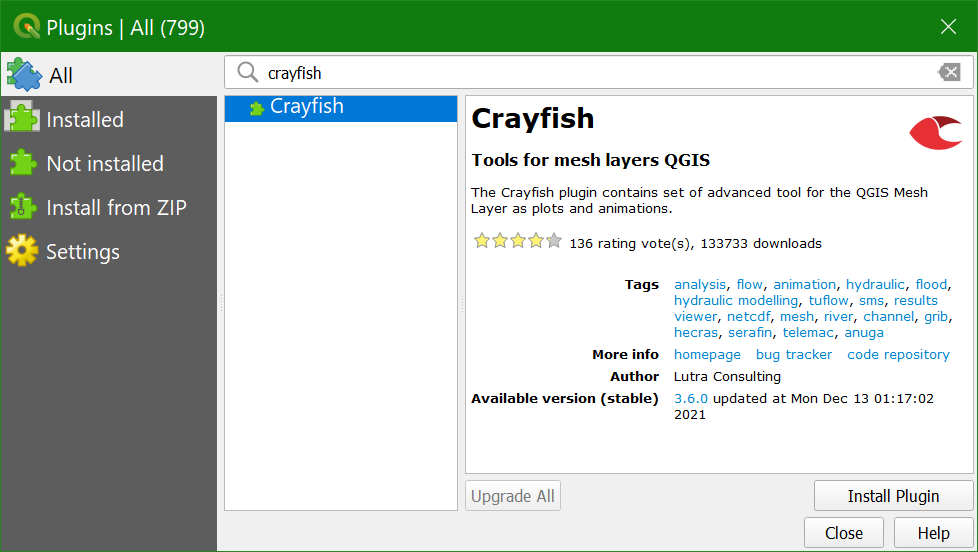
2. In the Processing Toolbox, go to Crayfish | Conversions | PCRaster LDD to GRIB.
3. In the PCRaster LDD to GRIB dialog, choose flowdirection as Input raster and flowdirmesh.grb as Output file (GRIB).
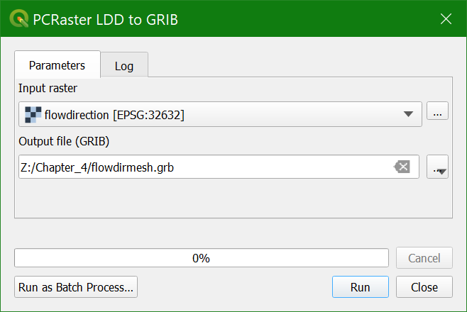
4. Click Run and Close to close the dialog.
5. In the Browser panel, expand the flowdirmesh.grb group (you might need to refresh the Browser panel with the  button) and drag the flowdirmesh layer with the mesh icon
  to the map canvas.
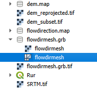
This might take some time. If the file is too large for your computer’s memory, you can get errors. In that case, you can clip the flowdirection layer to a smaller area and repeat the steps to convert the file to the mesh format.
When the map canvas shows a completely yellow layer, the flowdirmesh layer has been loaded and we can start styling it.
6. Select the flowdirmesh layer in the Layers panel and open the Layer Styling panel.
7. In the Layer Styling panel, go to the Datasets tab and click on  to disable contours and click on the arrow to enable vectors. You might need to make the panel larger to see the arrow.
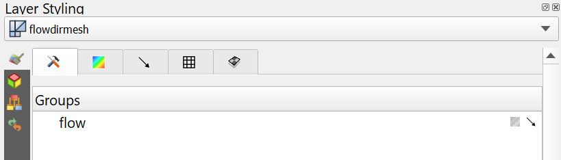
Now so many arrows are drawn in the map canvas that it turns black. Let’s tune the settings to improve this.
8. Go to the Vectors tab  and change the Arrow Length settings to Fixed and the Length to 2.00. Change the Color to dark blue.
9. Zoom in to see the flow direction with arrows.
10. Check the box to Display on User Grid to show the arrows fixed to a grid, e.g. with an X and Y Spacing of 10 px.
The settings are depending on your zoom level. Play with the settings to get a nice result. You can also try the other Symbology settings for visualization as Streamlines and Traces.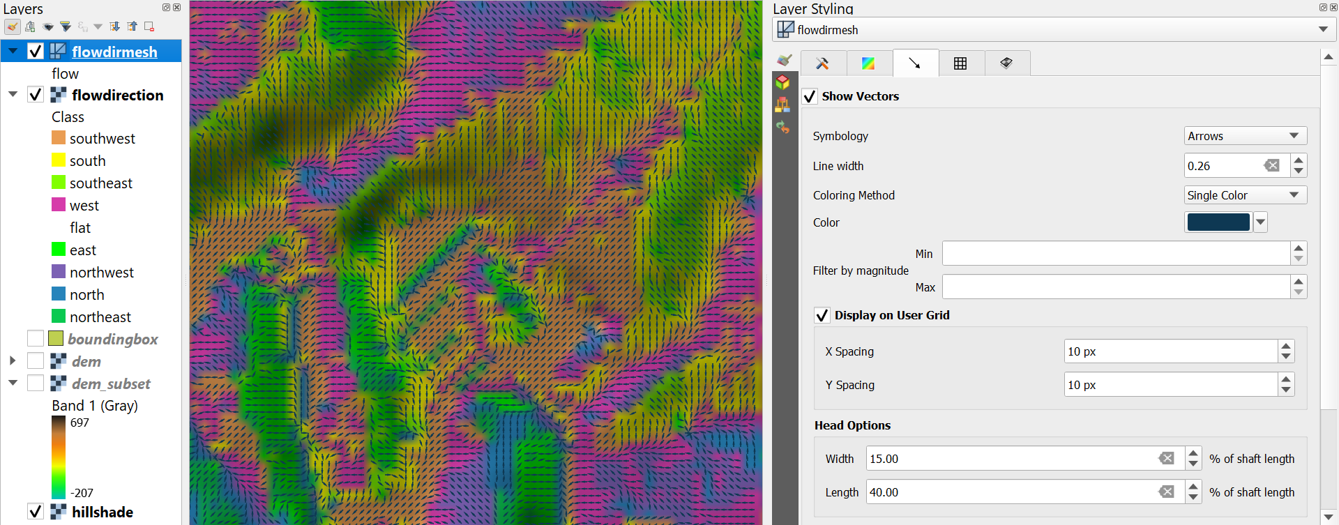
Watch this video to check the steps until this point:
7.2. Visualize Flow Direction in 3D
We can also visualize the flow direction using the QGIS 3D Map View.
1. In the main menu, choose View | New 3D Map View.

2. In the 3D Map view, click the Options
 button and choose Configure....
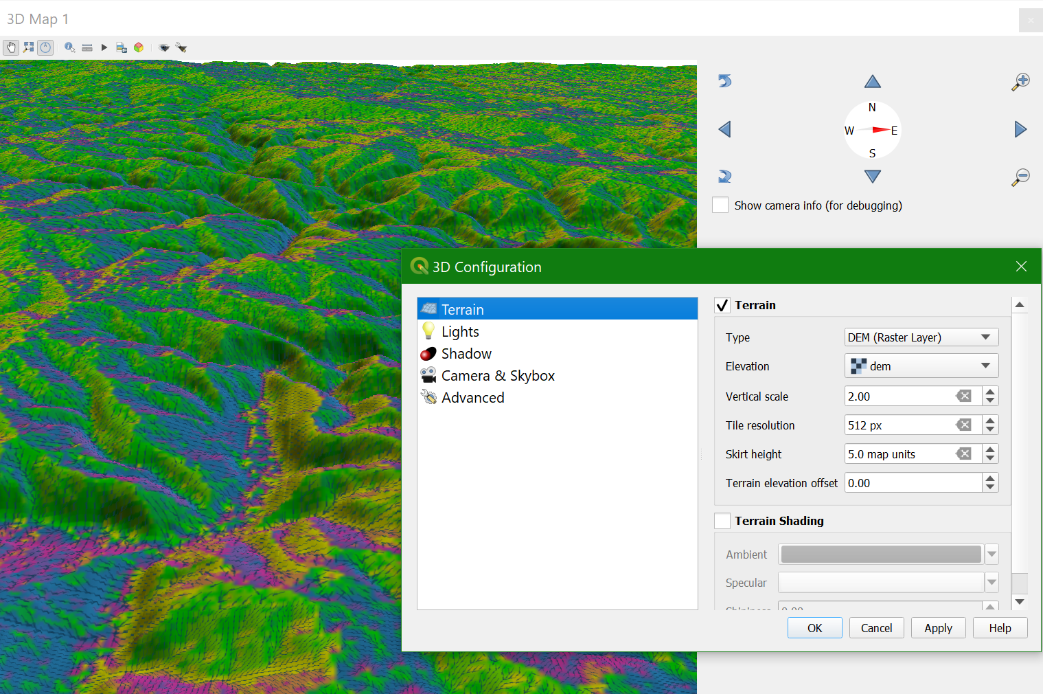
3. In the 3D Configuration dialog, go to the Terrain tab and change the Type to DEM (Raster Layer) and choose dem as Elevation. Click OK to apply the settings and return to the 3D Map view.
The 3D view will now start rendering. Try to navigate the scene with the different mouse buttons and the compass. You can change the Vertical scale, Tile resolution and Skirt height in the 3D Configuration to improve the visualization.
8. Delineate Streams
Now we have the flow direction we can proceed with delineating the streams.
First we'll calculate the Strahler Orders, then we'll calibrate the Strahler threshold to determine the streams.
8.1. Calculate Strahler Orders
Before we can derive the streams from the DEM, we need to determine what we consider streams. For this purpose we use the Strahler order. The higher the order, the bigger the stream.
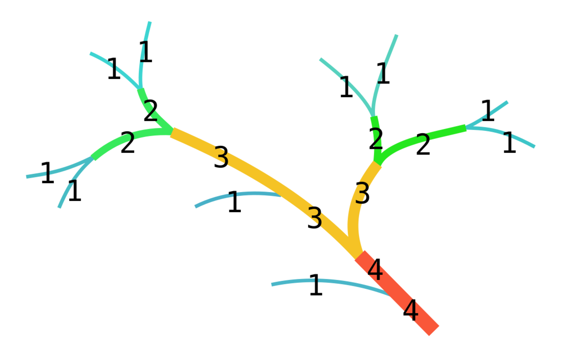
1. Close the 3D Map view and show only dem_subset with blended hillshade by unchecking the other layers in the Layers panel. Also zoom out to the full extent.
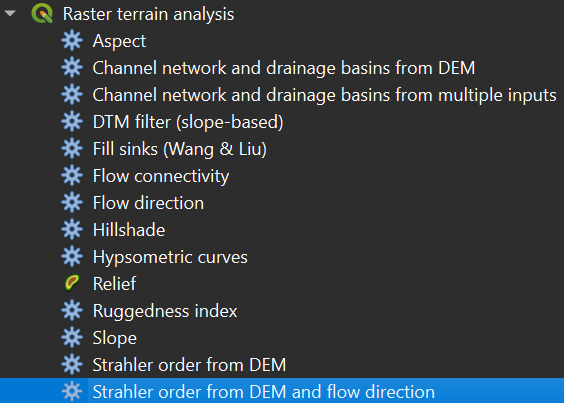
2. In the Processing Toolbox go to Raster terrain analysis | Strahler order from DEM and flow direction.
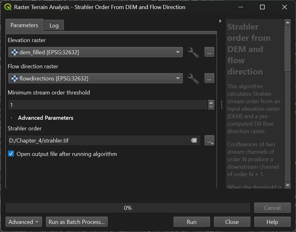
3. In the dialog, select dem_filled for the Elevation raster and flowdirections for the Flow direction raster. Use strahler.tif as the Strahler Order output filename, and click Run. Click Close when the algorithm is done.
To make more sense of the strahler layer we are going to style it.
- Is the Strahler order layer a Boolean, discrete, or continuous raster?
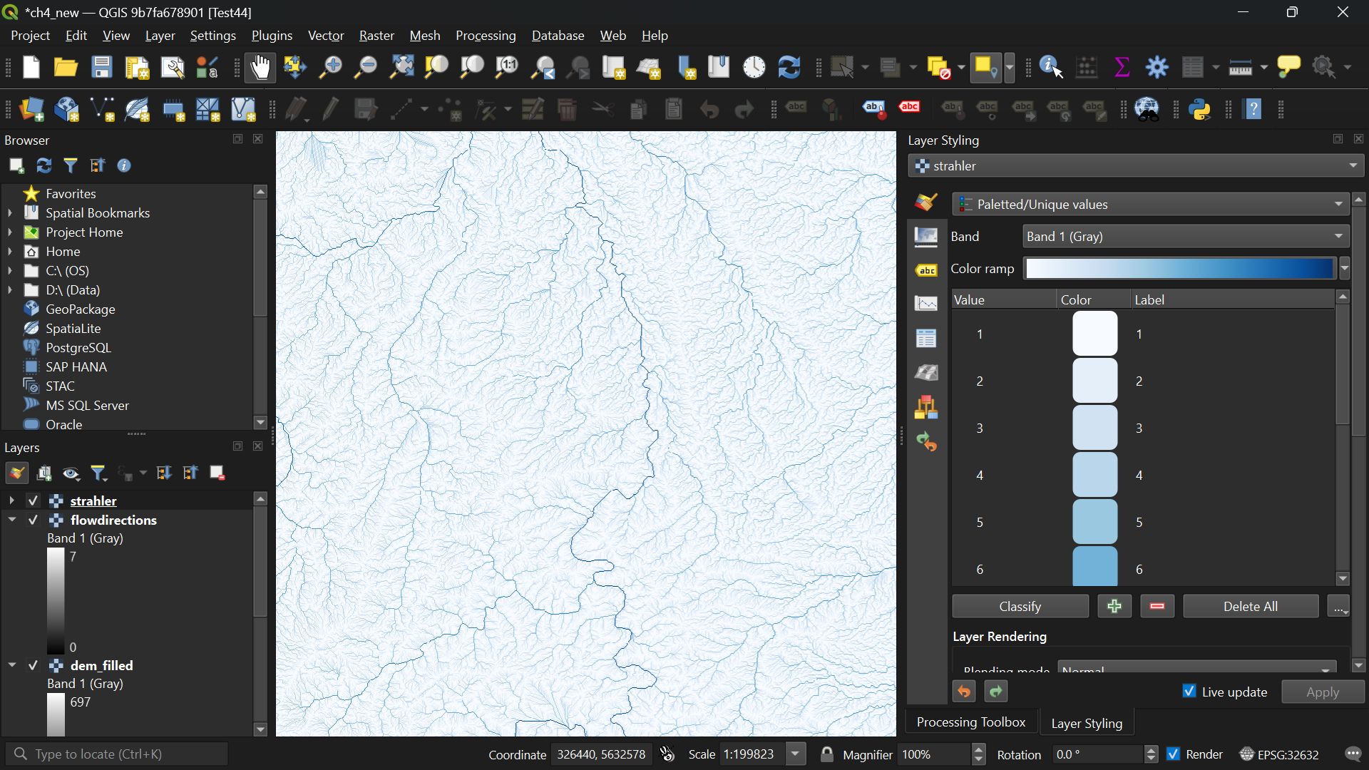
The Strahler order layer is a discrete raster, but the order of the classes is important. For discrete rasters in QGIS we use the Paletted/Unique values styling. The higher the Strahler order, the bigger the stream. So we will use a color ramp from white to blue.
4. Open the Layer Styling panel if you closed it before and make sure that the strahler layer is selected.
5. Choose Paletted/Unique values from the drop-down menu.
6. Click Classify.
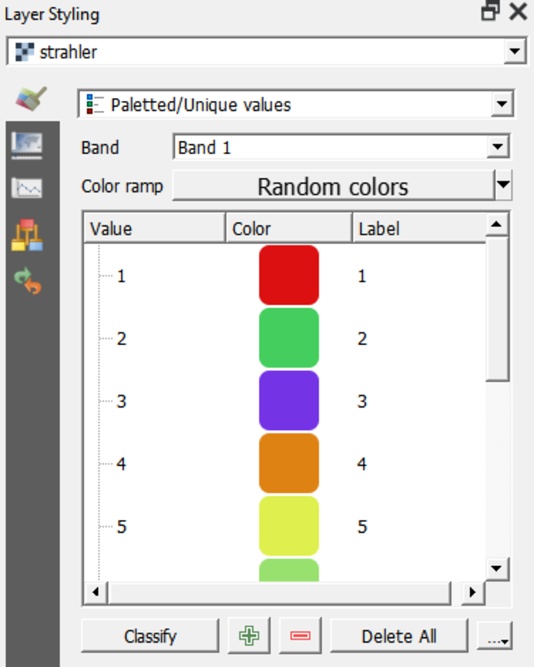
This assigns a unique, random color to each unique value in the raster.
7. Right-click on Random colors and choose Blues.
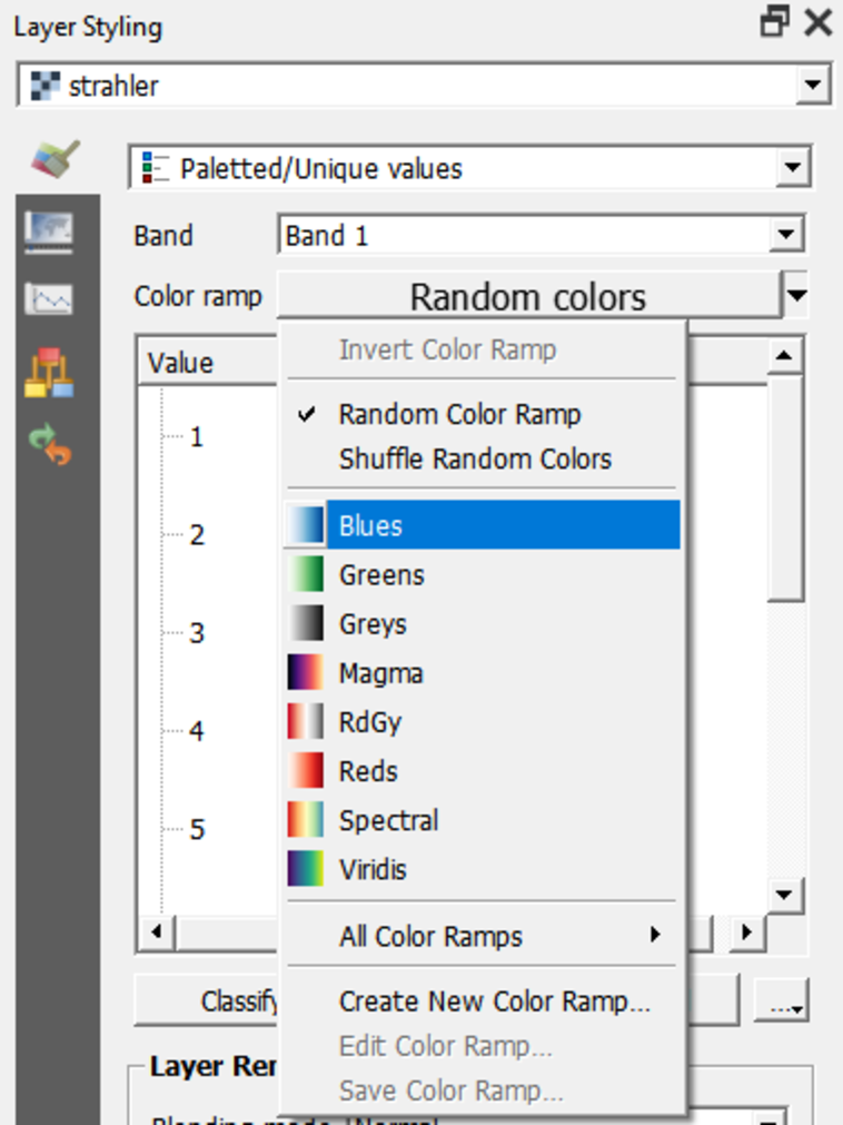
The strahler layer now shows in an intuitive way that the higher orders will be larger streams than the lower orders.
8.2. Calibrate Strahler Threshold to Determine Streams
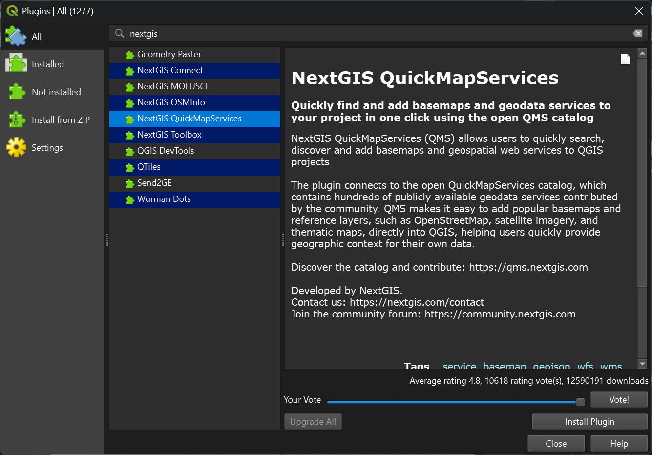
The next step is to apply a calibration procedure to determine which Strahler orders we consider to be streams. We will create boolean layers for Strahler orders larger than or equal to a threshold value. Each boolean layer will be compared with a reference layer. Here we will compare the Strahler orders with the rivers on OpenStreetMap. For areas where there is a lack of data in OpenStreetMap, you could use the Google Satellite. Both OpenStreetMap and Google Satellite layers can be found in the NextGIS QuickMapServices plugin.
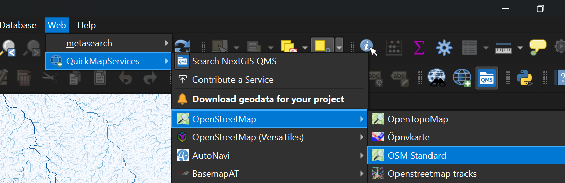
3. Fill in the dialogue as in the figure below. You can double click on a layer name to add it to the expression. Note that we check the box to Create on-the-fly raster instead of writing layer to disk, because we only need these layers for calibration purposes. Choose strahler >= 5 as the Layer name so we can compare results later. Click OK to run the calculation.
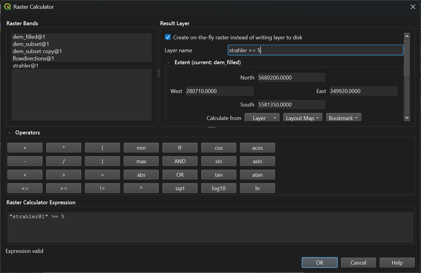
It is also good practice to style the strahler5.
4. Go to the Layer Styling panel and make sure that strahler >= 5 is selected.
5. Choose Paletted/Unique values from the drop-down menu.
This layer is boolean and therefore it has only pixels with values 0 and 1, but it also shows a nodata value. For our calibration it is important to make the ones blue and the rest of the pixels transparent so we can compare the raster with the streams on OpenStreetMap.
 to remove these classes.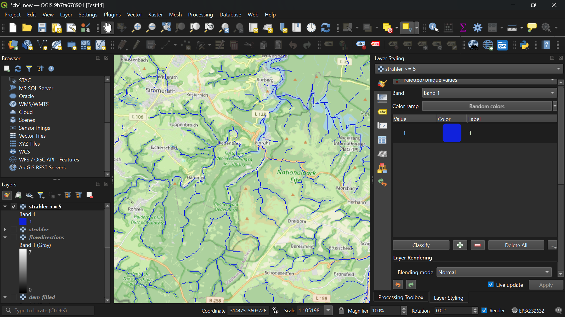
On the map canvas we can see now all streams larger than or equal to Strahler order 5 and we can compare them with the rivers on the OpenStreetMap.
8. Repeat the steps in this subsection for different Strahler order threshold values and determine the one that corresponds best with the rivers on OpenStreetMap. Remove the other boolean layers and save the final one as channels.tif.
Tip: You can copy the styles of the layers: right-click on a layer, choose Styles | Copy Style and then right-click on the target layer and choose Styles | Paste Style.
8.3. Calculate Channel Network
The next step is to calculate the channel network.
- In the Processing Toolbox, go to Raster terrain analysis | Channel network and drainage basins from multiple inputs.

2. In the dialog, choose dem_filled for the Elevation raster, flowdirections for the Flow direction raster, strahler for the Strahler order raster and the minimum treshold value that you found, for example 8, for the Minimum stream order threshold.
3. Only save the Channels result. Save it as channels.gpkg.
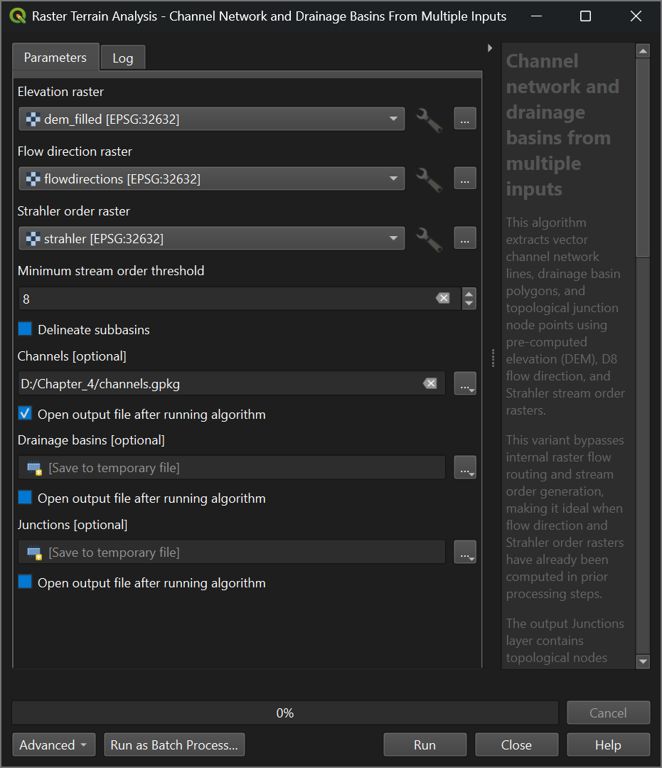
4. Click Run. Click Close after processing.
Next, we'll style the channels.
8.4. Styling the channels
Now we can style the channels vector layer to get a better understanding of the results. We will apply a styling in such a way that the lines get thicker with higher Strahler orders.
2. Open the Layer Styling panel and set the target layer to channels.
3. Keep the Single Symbol renderer, but change the Symbol layer type from Simple Line to Interpolated Line.
4. Change the Stroke Width to Varying Width. Set the Start value and End value to the ORDER field. Click the refresh  button to get the correct Min. value and Max. value. Change the Min. width to 0.30 Points and the Max. width to 1.00 Points.
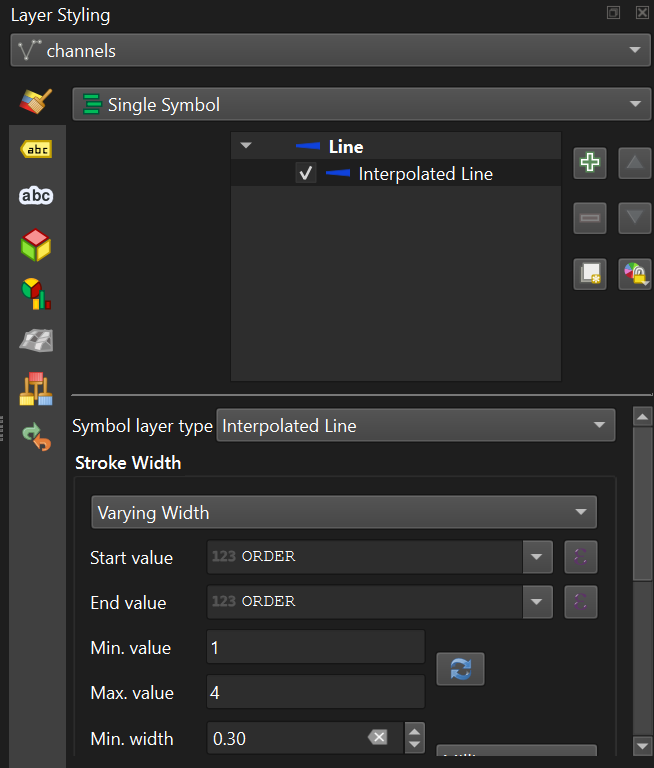
9. Under Color, keep the Single Color but change it to blue with an RGB value of 15 |66 | 220.
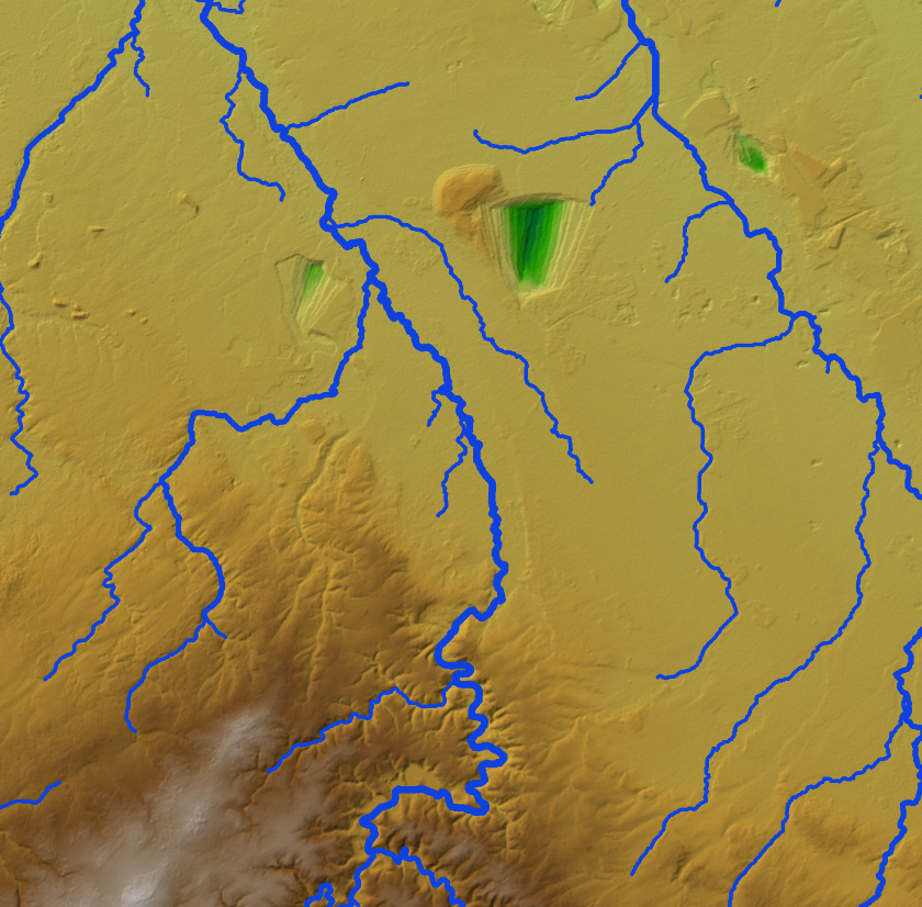
Your map should now resemble the figure below, showing the streams identified as having higher Strahler Orders are the main channels and the smaller ordered streams are tributaries.
9. Delineate the Catchment
A catchment is an extent or an area of land where surface water from rain, melting snow, or ice converges to a single point at a lower elevation, usually the exit of the basin, where the waters join another water body, such as a river, lake, reservoir, estuary, wetland, sea, or ocean. In order to delineate a catchment we need to have:
- the coordinates of our outlet in the same coordinate system as the map we are using
- the channel network that matches the flow directions as calculated from a hydrologically correct DEM
The outflow point of the Rur catchment is in Roermond, where the Rur enters the Meuse river (Maas in Dutch). The channel network that has been derived in the previous step is in the channels layer. We will however use the channelsstrahler raster layer, because we need to define the outlet exactly on a river pixel.
1. Make sure you have the channels raster layer is on top of the OpenStreetMap layer. You can style the channels layer with a blue ramp, so that the main channel appears in dark blue.
2. Look for the location where the Rur river flows into the Meuse. Note that on the OpenStreetMap the Dutch names are used, because it lies in the Netherlands. Rur is spelled as Roer and Meuse is spelled as Maas.
Note that the delineated channels are not corresponding well with the channels on OpenStreetMap. This can be for the following reasons: (1) Incorrect automatic delineation of streams, which can be caused by errors in the DEM or areas that are too flat, (2) Distortion due to (on-the-fly) reprojection and resampling, and (3) Human influence on the natural course of the channels. The catchment delineation, however, only works when the outlet is defined on a delineated channel, because that corresponds with our flow direction layer. Results can be improved by using different (parameters of) fill sinks algorithms or burning an existing vector layer of the stream network in the DEM.
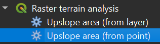
3. In the Processing Toolbox, choose Raster terrain analysis | Upslope area (from point).
4. In the dialog, choose dem_filled as Elevation. Check if the Method is set to Multiple flow direction, because D8 doesn't give good results in this case.
5. At Target point, click  . Now you can click on the outlet location in the map canvas. Choose a pixel on the delineated channel that is close to the real outlet of the Rur in the Meuse (step 2). Make sure you stay upstream of the junction, otherwise you will also delineate a part of the Meuse catchment, which is wrong.
6. Save the result as catchment.tif.
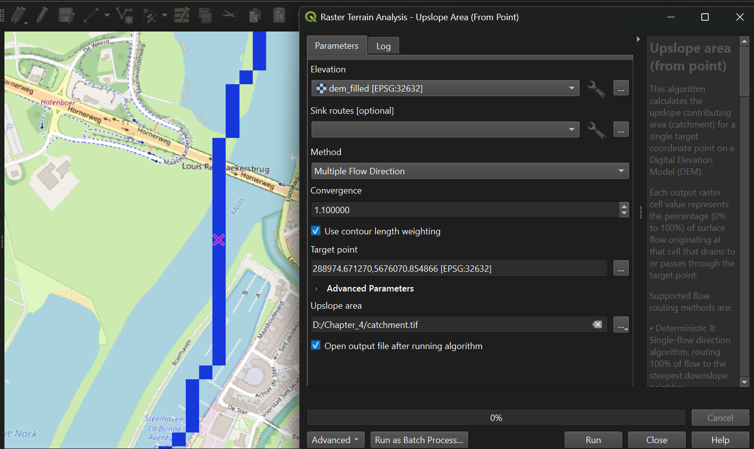
7. Click Run. Click Close after processing.
This should be the result.
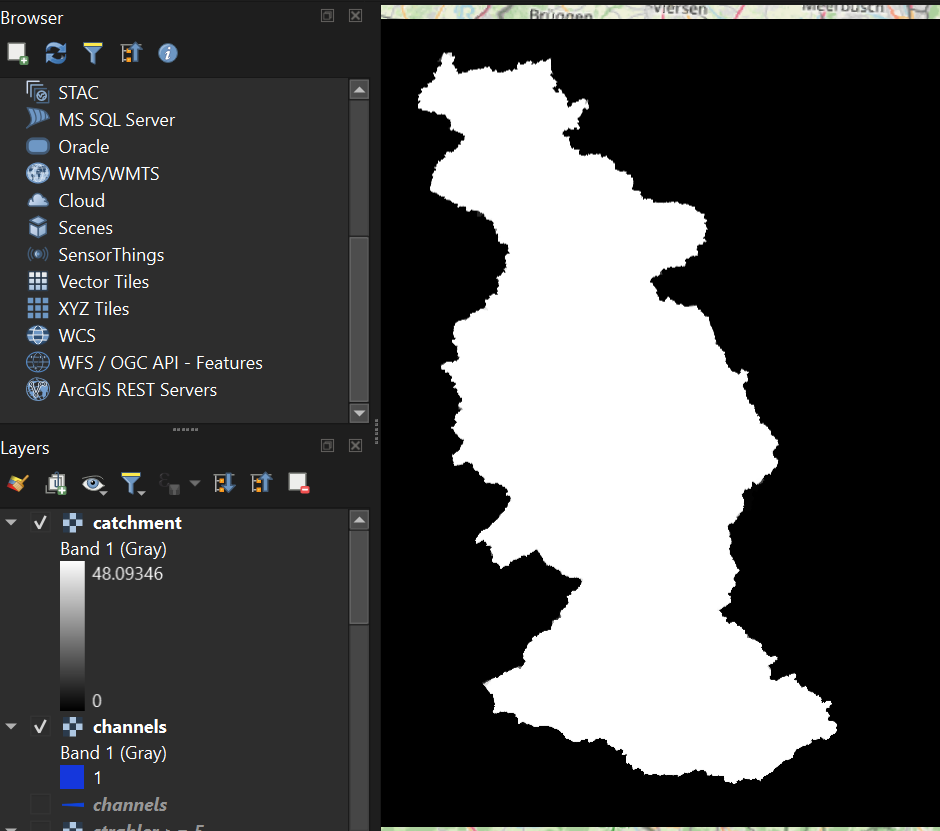
8. Go to the Raster Calculator and create a Boolean raster with True for cells larger than 0.
In order to overlay the catchment boundary with other data, it is better to convert it from raster to vector (polygon).
9. To convert the raster layer to vector, go to the main menu and choose Raster | Conversion | Polygonize (Raster to vector).
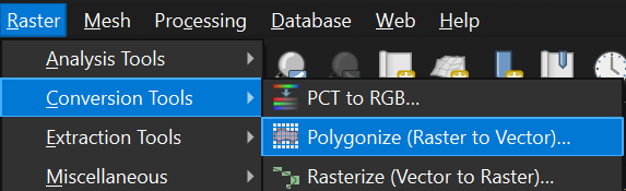
10. In the dialog choose the Rur_catchment raster as Input layer and save the result as Rur_catchment.gpkg.
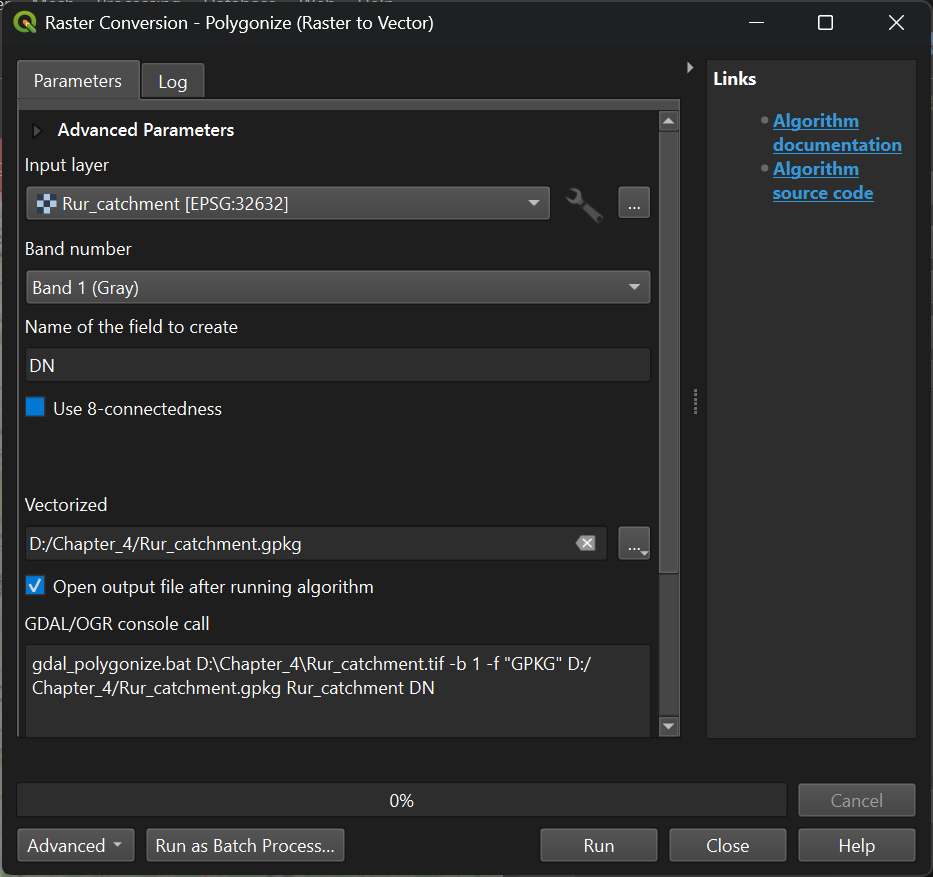
11. Click Run. Click Close after processing.
12. Look at the result. Also check the attribute table (right-click on layer name and choose Open attribute table).
In the catchment calculation, cells belonging to the catchment get a value of 1, while the other cells get a value of 0. During the conversion to polygons, it can happen that geometry errors are introduced. If you find more than one feature with a value of 1 this indicates a geometry error (incorrect topology), because the boundary of the polygon makes a loop (see figure below). This can give errors when we use the polygon for geoprocessing. You can fix those errors with the fix geometry tool in the Processing Toolbox.
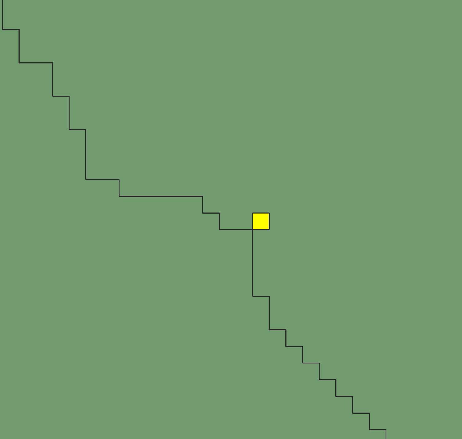
Of course we are only interested in the catchment area, so we have to remove the outside polygon.
13. Close the attribute table.
14. In the toolbar, click the Select feature by Area or Single Click tool .
15. Click on the catchment polygon, so it becomes yellow.
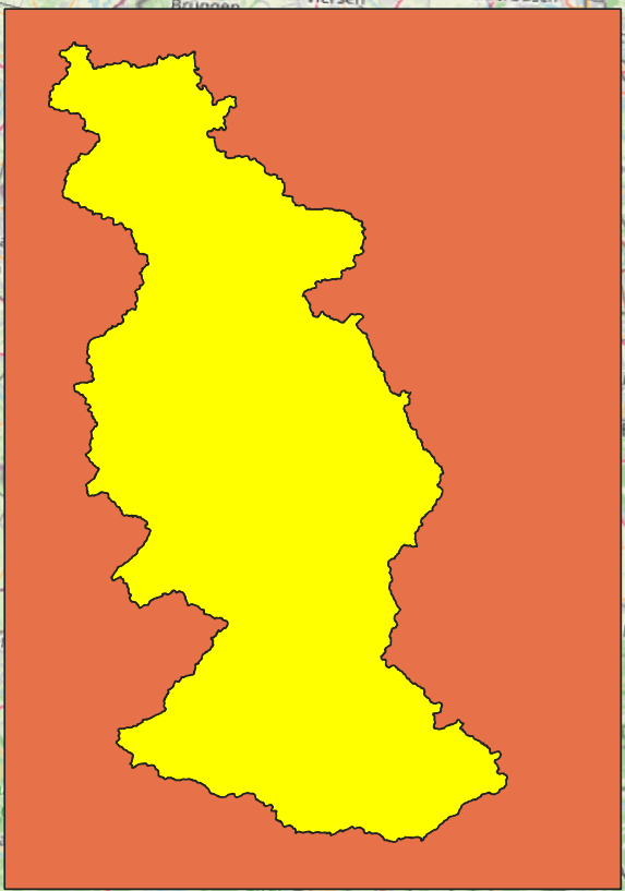
We want to keep this polygon, but remove the other ones.
10. In the toolbar. click the Invert Feature Selection tool .
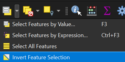
Now the other polygons are yellow:
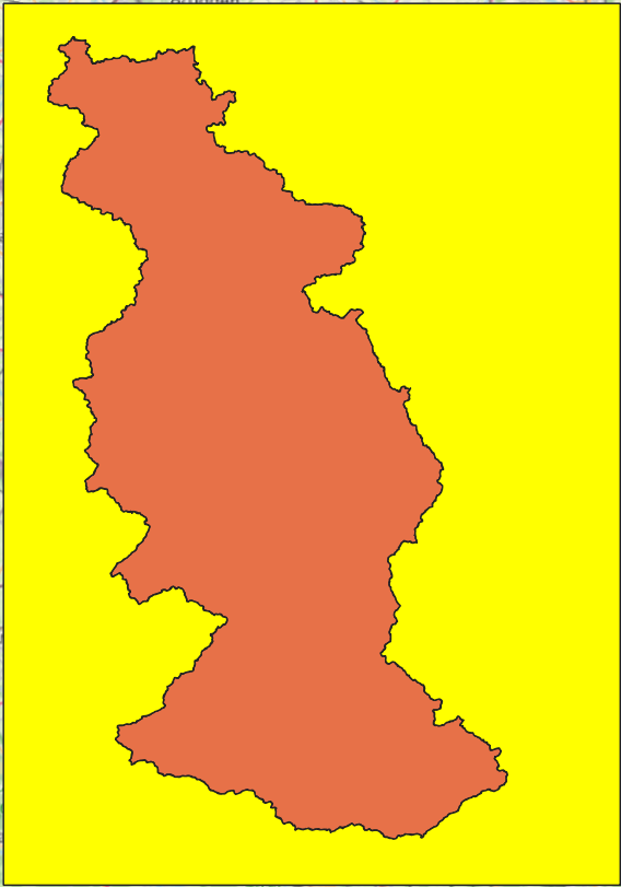
11. Click  to toggle to editing mode.
12. Click  to delete the selected polygons.
13. Confirm that you want to delete the features.
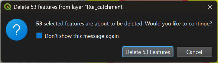
14. Toggle off editing by clicking again, and save the changes.
15. Now remove all unnecessary layers from the layers list so that we have only channels, Rur_catchment, dem_subset, hillshade and OpenStreetMap (in that order).
10. Clipping layers to the catchment boundary
For visualization, it is nicer to clip the layers to the boundary of the catchment.1. Let’s first clip the channels vector layer to see only the streams that are inside the catchment. Go to the main menu and select
Vector | Geoprocessing Tools | Clip...
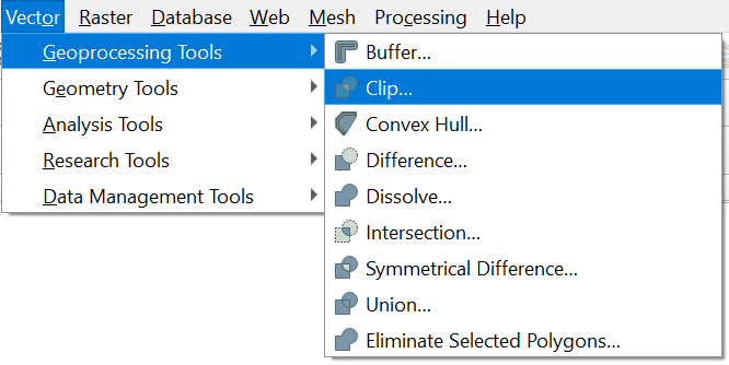
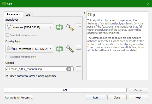
2 .Fill in the dialog as in the figure below to use the catchment layer as a "cookie cutter" to clip the Input layer channels to the boundary of the Overlay layer Rur_catchment. Call the Clipped layer Rur_channels.shp. Click
Run to run the tool. Click Close to return the main screen.
You'll probably get this error:

This is caused by geometrical errors in the channels layer. Let's fix this.
3. Click Close to close the Clip dialog.
4. In the Layers panel, select the channels layer.
5. In the toolbar of the Processing Toolbox, click  to Edit Features In-Place.
Some tools support this. For those tools, it is not necessary to save the result into a new layer.
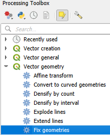
6. Choose Vector geometry | Fix geometries.
7. In the Fix geometries dialog, keep the default Repair method and click Modify All Features.
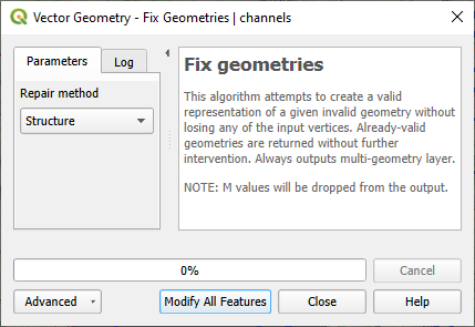
8. Click Close to close the dialog.
9. In the toolbar, click  to toggle off editing mode and save the result.
10. In the toolbar, click  to unselect the lines. Also click
  in the Processing Toolbox to toggle off in-place editing.
Now we can repeat the clipping. There's an easy way to redo operations by using the history.
11. In the toolbar of the Processing Toolbox, click  to open the Processing History dialog.
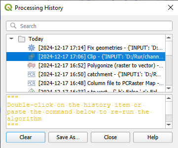
12. Search for Clip and double click to re-open the dialog.
You'll see that the Processing History stored the input layers and output file name that you had used before in the dialog.
13. Click Run.
Now the Clip tool runs without errors.
14. Click Close to close the dialog. Also close the Processing History dialog.
We can easily copy the styles from channels to Rur_channels.
15. Right-click on the channels layer and choose Styles | Copy Style | All Style Categories.
16. Now right-click on Rur_channels and choose Styles | Paste Style | All Style Categories.
17. Remove channels from the layers list and make sure that Rur_channels layer is at the top of the list.
11. Styling the Resulting Catchment Area
To show the results of your analysis you can use a technique named Inverted Polygon Shapeburst Fills to focus attention on the Rur Catchment.
1. Open the Layer Styling panel by clicking the  button. Set the target layer to Rur_Catchment.
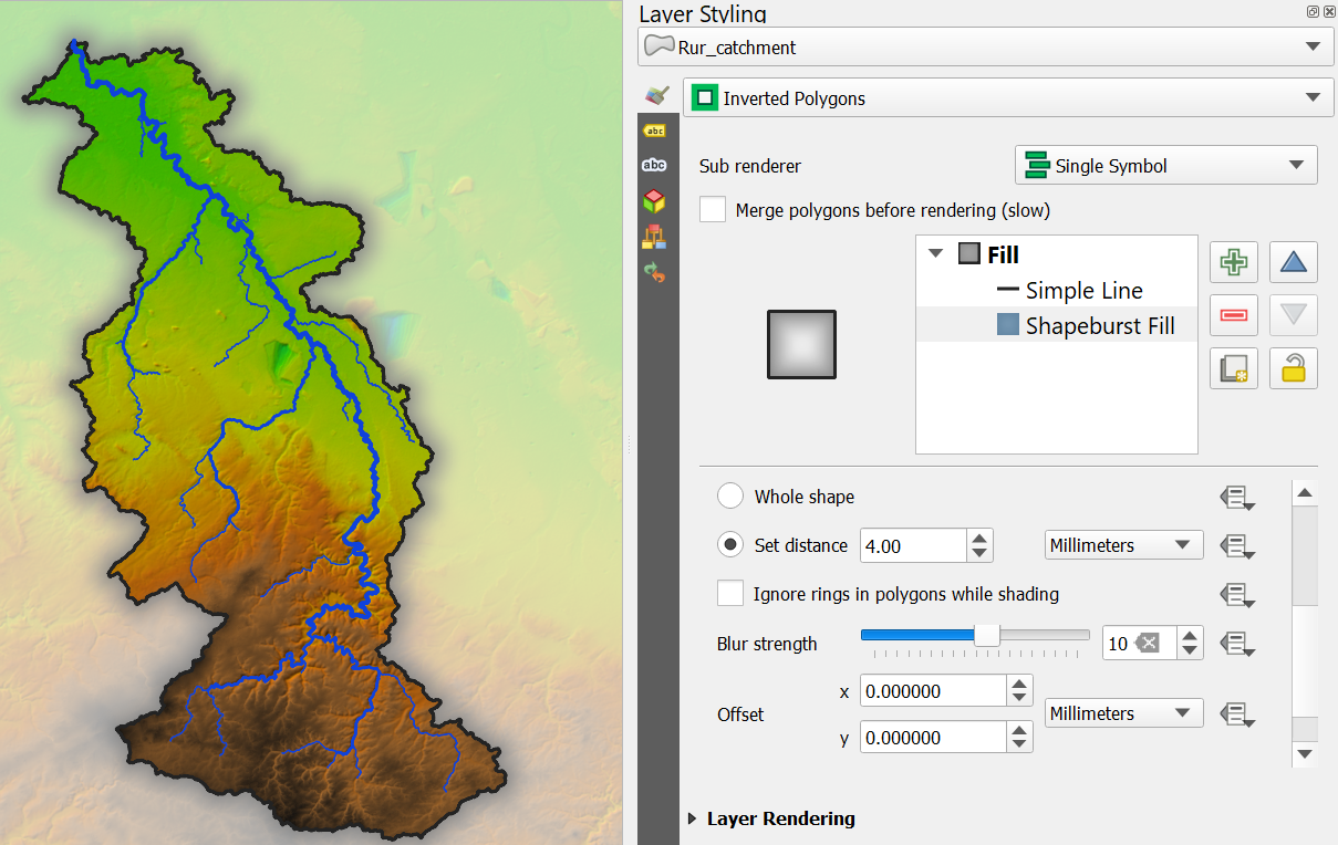
2. Change from a Single symbol renderer to an Inverted polygons renderer. This renders the data as the inverse of its geometry, i.e. you'll style everything outside of the polygon. This creates a mask around the Rur valley.
3. Next, select the Simple Fill component. Then change the Symbol layer type to Shapeburst fill. In the Gradient colors section use the default Two color method. Change the first color to an RGB value of 135 | 135 | 135. Change the second color to white with an opacity of 65%.
4. In the Shading style section, click the Set distance option and set the distance to 4 mm and increase the Blur strength to 10.
5. Finally at the top of the Layer Styling Panel select the Shapeburst fill component.
7. Click the Add symbol layer  button. Change the new Simple fill renderer to a Symbol layer type of Outline: simple line. Give it a Color of
black and a Stroke width of 0.46 mm.
button. Change the new Simple fill renderer to a Symbol layer type of Outline: simple line. Give it a Color of
black and a Stroke width of 0.46 mm.
This gives us the nicely styled basin as shown in in the figure below.
Watch this video to check the steps:
12. Storing the Data in a GeoPackage
To keep the data together and enable easy distribution, it is good to save the layers as a GeoPackage.
1. In the Processing Toolbox look for the Package Layers tool.
2. In the Package Layers dialogue click the  and select all layers. Note that these are only the vector layers.
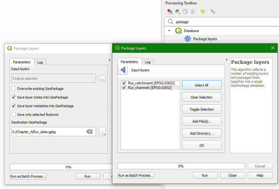
3. Save it as Rur_data.gpkg and click Run and Close when it's done. By default it will also save the styles.
4. We can add the raster layers from the Browser panel. Simply drag the raster layers (in our case dem_subset) to the Rur_data.gpkg. You might need to refresh the Browser panel to see the GeoPackage.
The layers in our project still refer to the the GeoTIFFs and the shapefiles. Let's change that in such a way that they will be linked to the layers in our GeoPackage.
5. Select a layer in the Layers panel and right-click. From the context menu, select Change Data Source.... Select the corresponding layer in the GeoPackage.
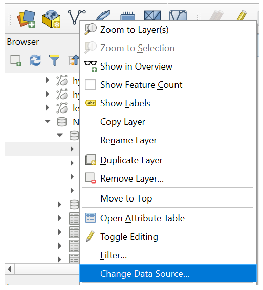
6. Repeat this for all layers (except of course the OpenStreetMap layer).
Now we can save the project to the Rur_data.gpkg with the correct paths.
7. In the main menu choose Project | Save to | GeoPackage...
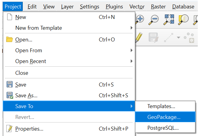
8. In the pop-up, browse to the Rur_data.gpkg at Connection and name the Project Rur. Click OK to save the project in the GeoPackage.
The end result should now look like this:
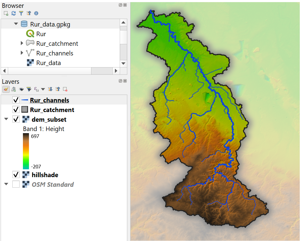
Watch this video to check the steps of this section:
13. Conclusions
In this lesson you have learned to:
- find and download SRTM DEM tiles from the EarthExplorer website
- mosaic raster layers into a virtual raster
- reproject rasters
- create subsets of rasters
- fill sinks in a DEM
- calculate and style flow direction raster layers
- calculate Strahler orders
- delineate streams
- delineate catchments
- style layers for visualising catchments