Tutorial: WebODM
| Site: | OpenCourseWare for GIS |
| Course: | Processing drone images with WebODM |
| Book: | Tutorial: WebODM |
| Printed by: | Guest user |
| Date: | Saturday, 4 July 2026, 7:16 PM |
Table of contents
- 1. Introduction
- 2. Theory
- 3. What can we do with WebODM?
- 4. Starting with WebODM
- 5. Add a new project
- 6. Select drone images
- 7. Review settings
- 8. Start Processing
- 9. Viewing results in WebODM in 2D
- 10. Viewing results with the 3D View
- 11. Download Assets
- 12. Use the results in QGIS
- 13. Process the images of 2020
- 14. Compare results in QGIS
1. Introduction
In this tutorial you'll learn how to use WebODM.
WebODM is a user friendly web interface to OpenDroneMap (ODM). ODM is an open source processing engine for processing drone images and creating point clouds, 3D models and orthophotos.
Learning objectives
- Use WebODM installed on a server
- Upload your drone images to WebODM
- Evaluate the most important task options
- Generate point clouds
- Generate Digitial Surface Models
- Generate orthophotos
- Visualise and evaluate results in WebODM
- Visualise and evaluate results in QGIS
- Compare results of different moments in time in QGIS
2. Theory
Watch this video for the theory and an overview of the tutorial.
3. What can we do with WebODM?
WebODM is a user friendly web interface to ODM.
These are the features of WebODM:
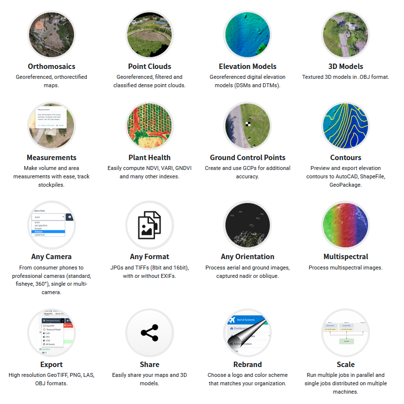
Source: website WebODM
In this tutorial we'll cover:
- orthomosaics
- point clouds
- elevation models
- measurements
- export
- share
4. Starting with WebODM
WebODM is open source and you can install it on your own computer or on a server. You can also get paid services to make things easier.
You can find all options at the WebODM website. We'll not cover how to install WebODM on your computer, but if you're interested, you can check these instructions.
1. Go with your internet browser to your WebODM page.
2. Use the credentials to log in.
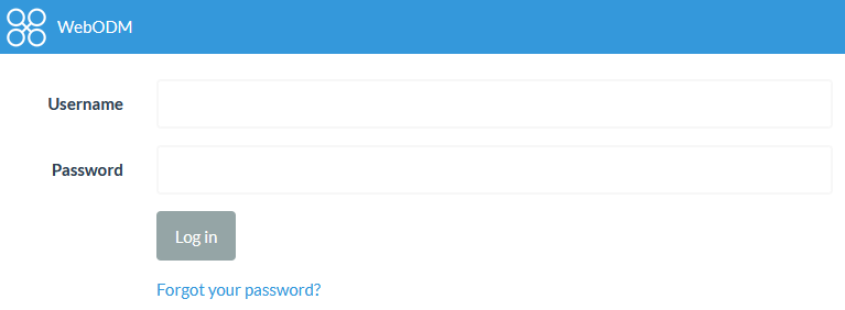
3. Click Log in
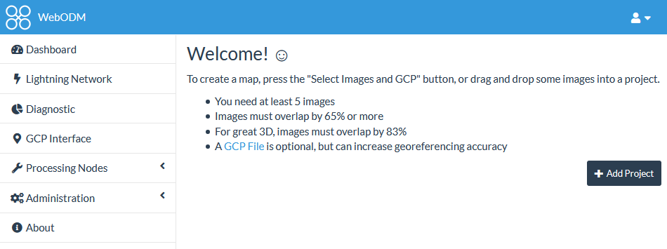
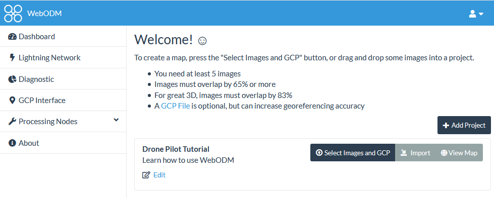
Now you're logged in at WebODM and you can see the Dashboard page:

In the next chapter we're going to create our first project.
5. Add a new project
The first step is to add a new project to your account.
1. Click Add project.
2. In the popup that appears, give your project a name and a description.
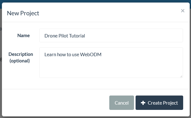
3. Click Create Project.
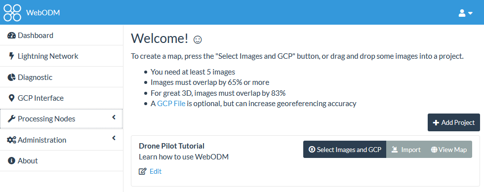
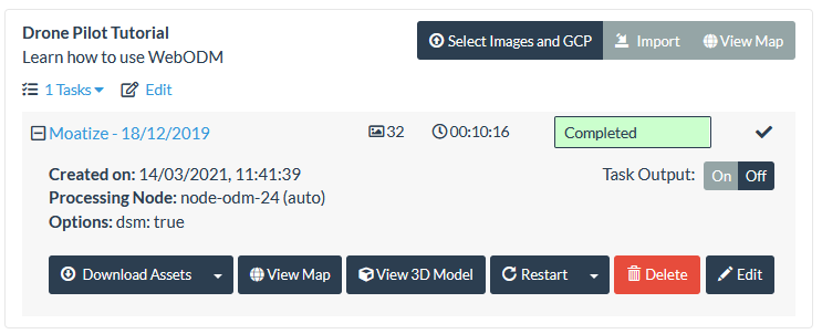
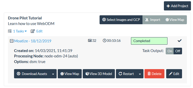
Now you see the project added to your Dashboard page:
You can still change the name and description by clicking Edit.
In the next chapter we're going to add the drone images.
6. Select drone images
In this chapter we're going to add the drone images.
We have prepared a dataset from flights over an agricultural area in Moatize (Mozambique) for this tutorial. The dataset contains:
- Drone images taken on 19 December 2019 (Moatize_Flight_20191219.tar.gz)
- Drone images taken on 22 January 2020 (Moatize_Flight_20200122.tar.gz)
- Boundary of an area of interest (bdry.zip)
4. In the File Upload dialogue, select all images (Ctrl-A is a useful shortcut to select all) and click Open.
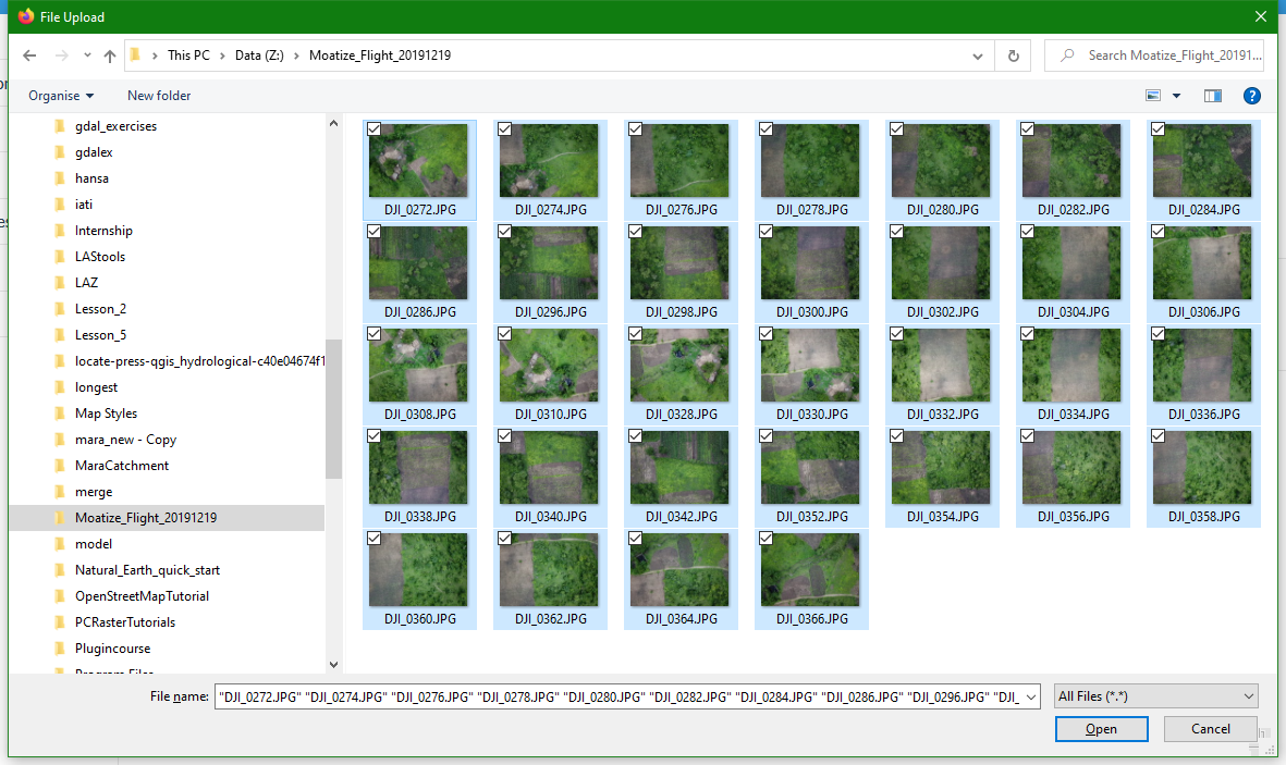
Alternatively, you can drag and drop files in WebODM. You can add more images from different folders by clicking Select Images and CGP again.
Now you see in the Dashboard that you've selected 32 files.

In the next chapter we're going to look at the settings in this dialogue.
7. Review settings
Now we have selected the 32 drone image we need to review the settings for creating this new Task in your Project.
WebODM reads the metadata from the images. The metadata is stored in as EXIF tags in the JPG files. EXIF stands for Exchangeable Image File Format. The tags can include information of the location where the picture was taken. This information comes from the GPS of the drone.
Images with geolocation information in the EXIF tags can be used to produce georeferenced orthophotos and elevation models. If location info is missing you can still create point clouds and 3D models, but it's not possible to create georeferenced orthophotos and elevation models. Later we'll briefly discuss how to add Ground Control Points in WebODM to still use those images for producing georeferenced orthophotos and elevation models.
Let's look at the different settings in the dialogue.
Name
The default name of the task is generated by WebODM by using the EXIF location and time data. The coordinates were used to look up the place name.
You can edit the name if needed. Here we keep the default name.
Processing Node
This the node where the calculation takes place. Your account is set up with a specific calculation node (you can see it when you use the dropdown menu), so you can keep this on Auto. In another setup where you have multiple processing nodes available you can manually choose the one you want to use or use Auto to automatically select the node with the least number of running tasks.
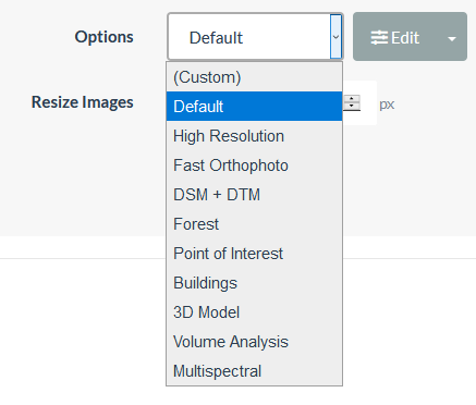
Options
- Default: create point cloud, orthophoto and DSM
- High Resolution: provides a higher resoltion output, but processing time will be longer
- Fast Orthophoto: if you're interested in an orthophoto only
- DSM + DTM: will generate a DTM besides a DSM
- Forest: will have a higher number of points and a higher quality to represent forests better
- Point of Interest / Building: better mesh representation to deal with man made structures
- 3D model: improved mesh
- Volume Analysis: improved DTM and DSM for volume calculations
- Multispectral: includes parameters for multispectral images, such as radiometric calibaration
Resize images
You can reduce the size of all images by changing the settings here. This is useful to lower the amount of memory used and to increase the processing speed. This is of course a trade off with the quality of the results. Here we're not going to resize the images, because that has already been done for the purpose of this tutorial.
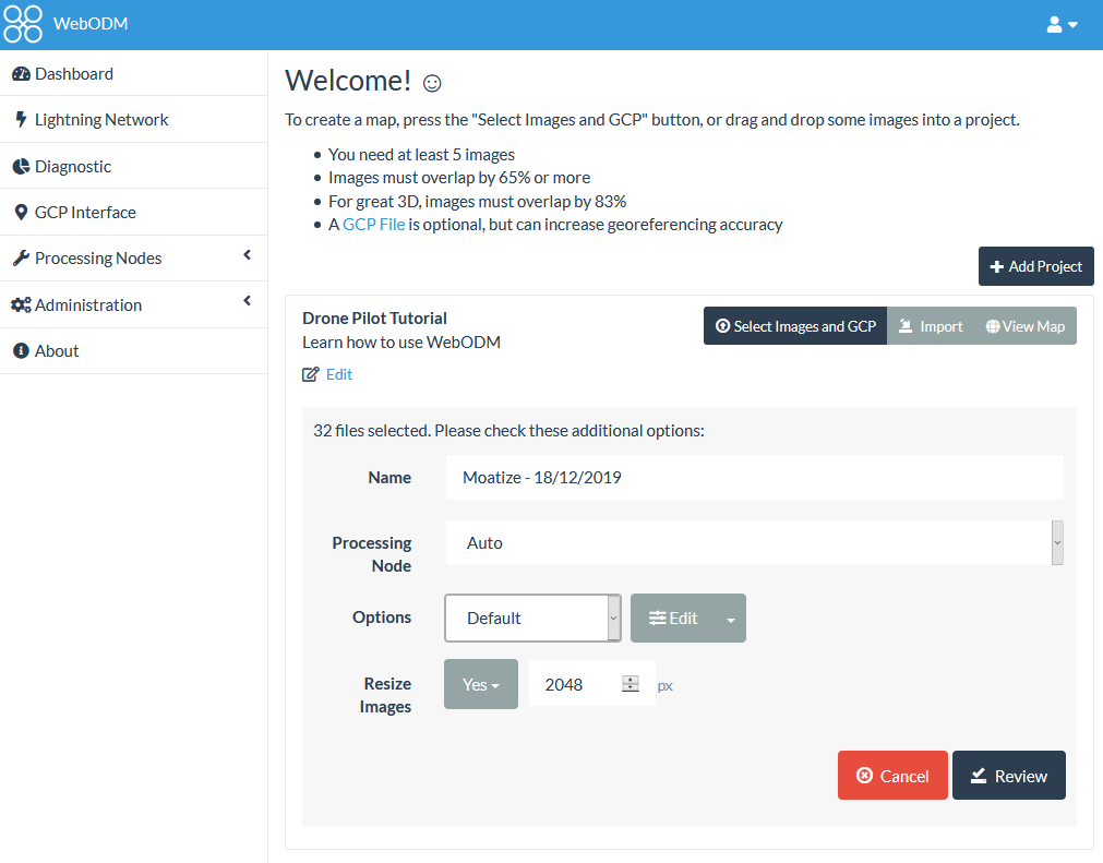
1. Select for Resize Images No.
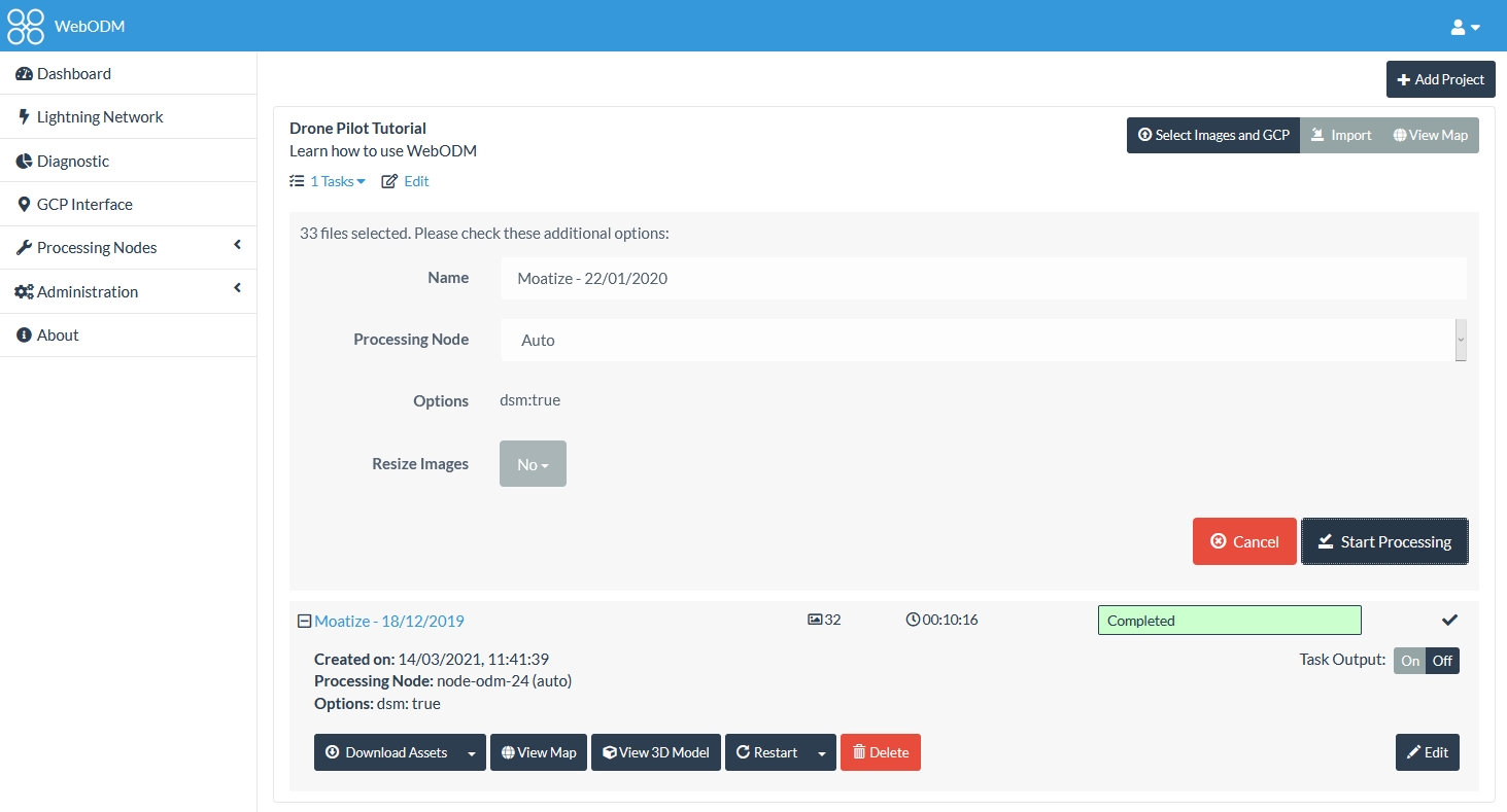
Now your setting should be like the screenshot below.
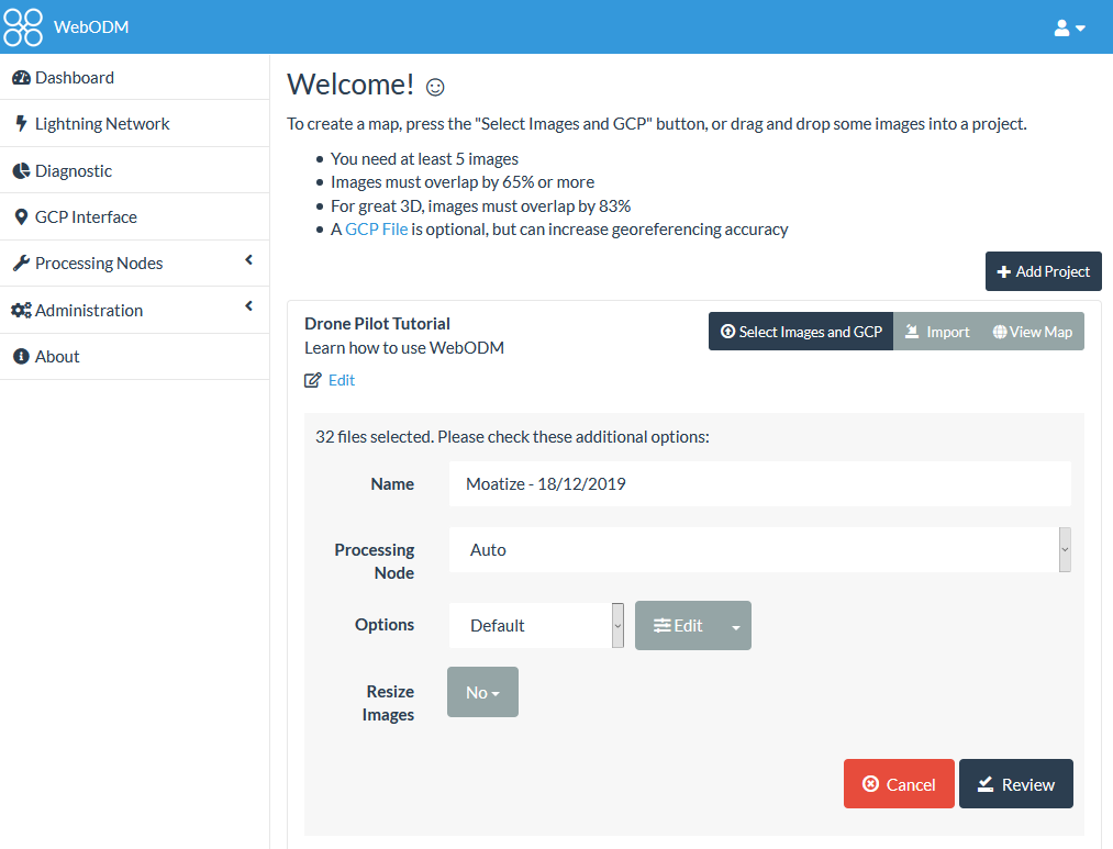
2. Click Review to proceed.
In the next chapter we're going to process the images.
8. Start Processing
In this chapter we're going to process the images.
1. Review if the settings are like the screenshot below. Click Cancel to make corrections if needed.
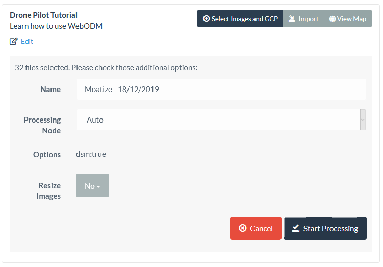
2. If the settings are correct, click Start Processing.
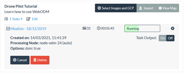
Now the task is executed, which will take a bit.
In the mean time we'll explain what is happening now.
First your images are uploaded to the correct folder on the server. Next, the images are sent to the selected processing node. These two steps are needed, because the processing nodes can be distributed over severall remote computers and the images need to be available at the node for further processing. Then the task is run on the node and the Dashboard will show the progress, including the elapsed time.
When the processing task is completed, we'll proceed with the next chapter of the tutorial.

9. Viewing results in WebODM in 2D
Once the processing of our task has completed, we can view the results in WebODM. Later we'll download the results and visualse them in QGIS.
Let's first have a look at our result in 2D.
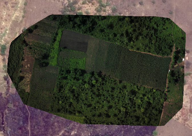
9.1. View orthophoto
Let's first have a look at the produced orthophoto.
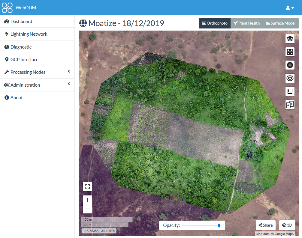
1. Click View Map.
The WebODM interface now shows the orthophoto with Google Maps Hybrid as a backdrop:
2. Inspect the results by:
- Changing the Opacity with the slider at the bottom of the screen.
- Compare the results with different base maps using the
 icon from the panel on the right of the screen.
9.2. Add vector data
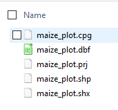
 icon in the panel on the right side of the screen to add the zipped shapefile.
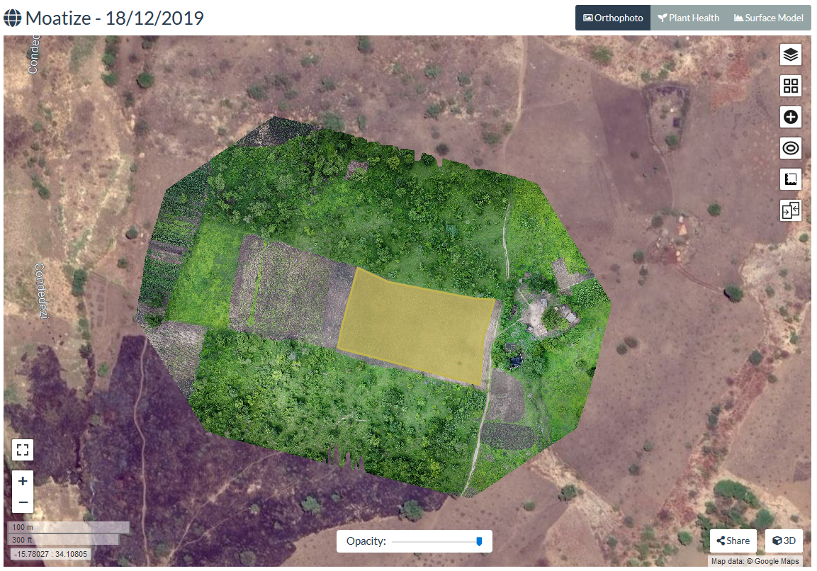
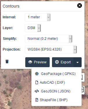
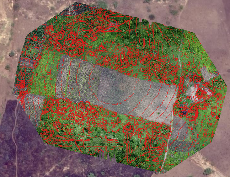
9.3. Derive contour lines
 icon in the panel on the right side of the screen.
- The interval (equidistance) of the contour lines
- The layer from which it is derived. In our case we can only choose DSM, because the default processing that we used doesn't produce the DTM.
- Degree of simplification
- Output projection
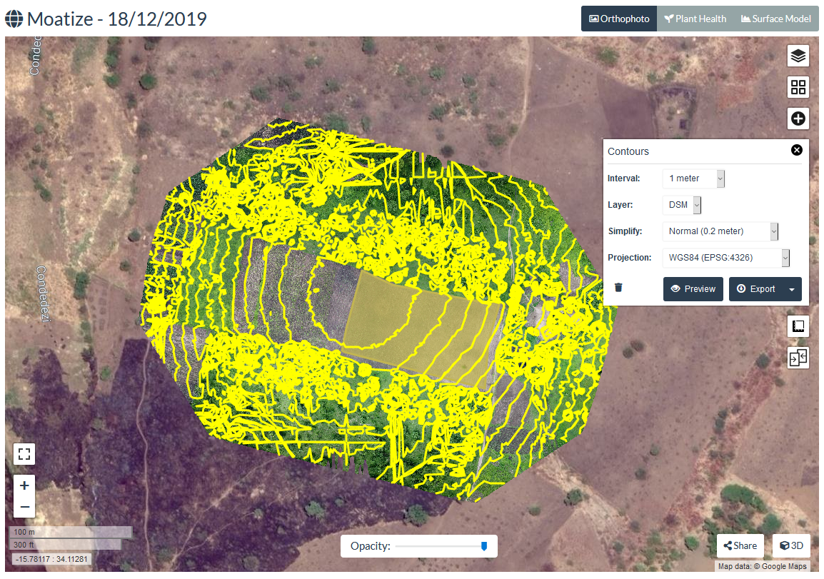
- What can you tell about the shape of our field of interest?
 icon to remove the preview.
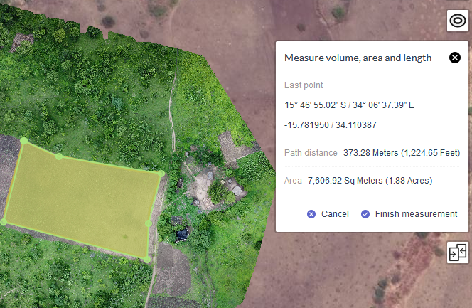
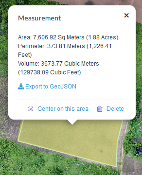
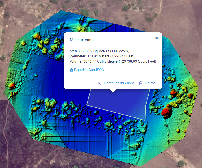
9.4. Measure length, area and volume
 icon in the panel on the right of the screen.
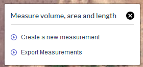
9.5. View surface model in 2D
In the 2D View we can also visualise the derived DSM
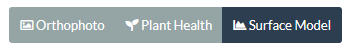
1. In the upper right of the screen click on Surface Model.
This will show the DSM of the area:
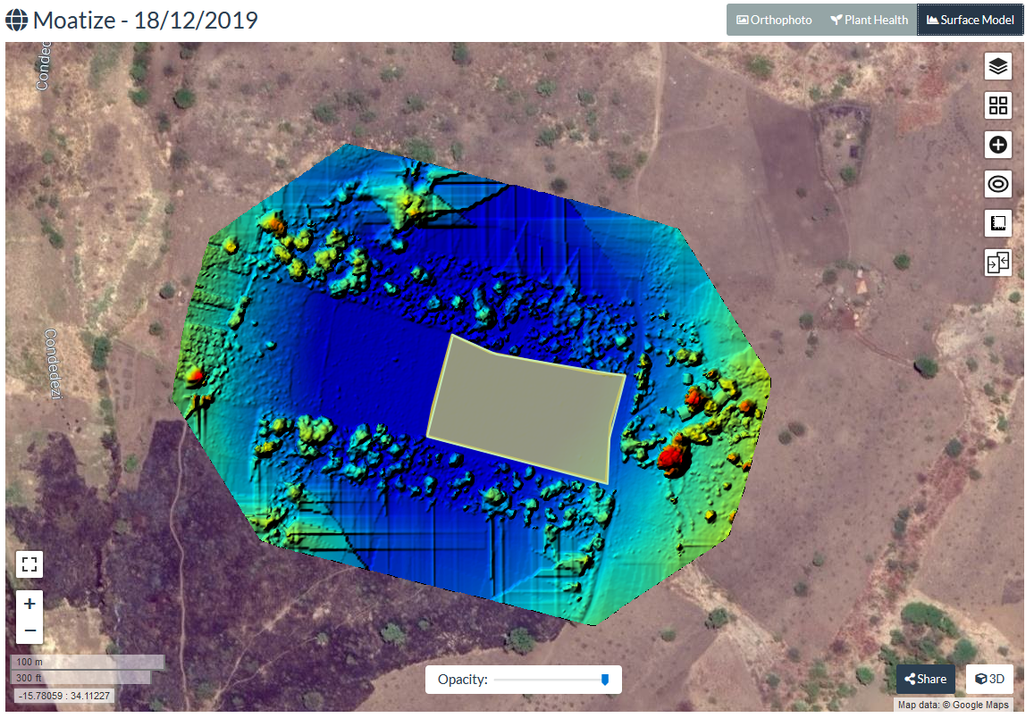
Now part of our view is covered by the polygon of our field of interest. Let's hide it.
2. Click on the  icon.
icon.
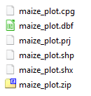
Here we can control which layers to visualise. We can for example switch off the polygon (maize_plot.zip) and add the camera locations where the drone made the pictures.
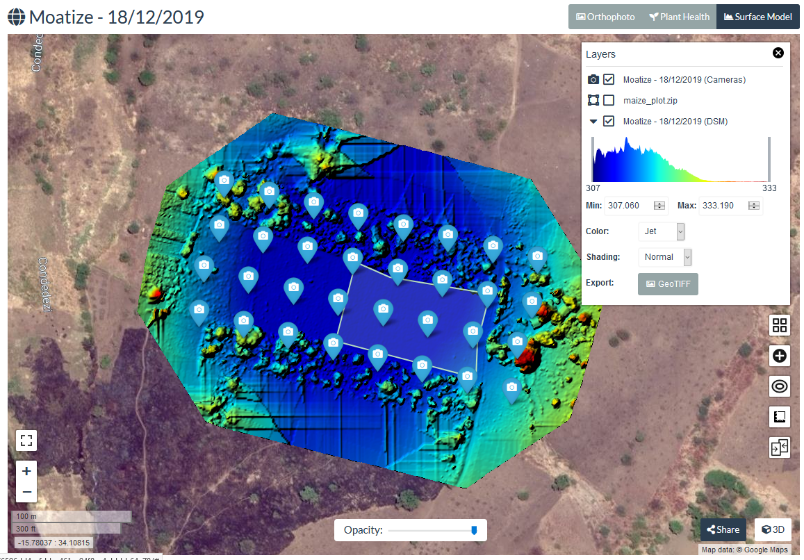
It also shows the elevations in a frequency histogram.
Under Color you can choose different colour ramps. With Shading you can change the shading of the elevation. You can also export the image as a GeoTiff to use in GIS.
3. Play with the color and shading settings.
4. Delete the measurement polygon that we have created earlier by clicking on it and choosing delete in the popup.
5. If you're happy with the result, you can click  to share the link with others. People with the link can only view your result in an interactive way.
In the next chapter we'll explore the 3D View.
10. Viewing results with the 3D View
In the previous chapter we have explored the 2D View of WebODM. Here we'll have a look at the 3D View.
1. Go to the 3D View. You can do this in different ways:
- If you are still in the 2D View, click
 to switch to the 3D View.
 - If you are in the Dashboard, click View 3D Model.
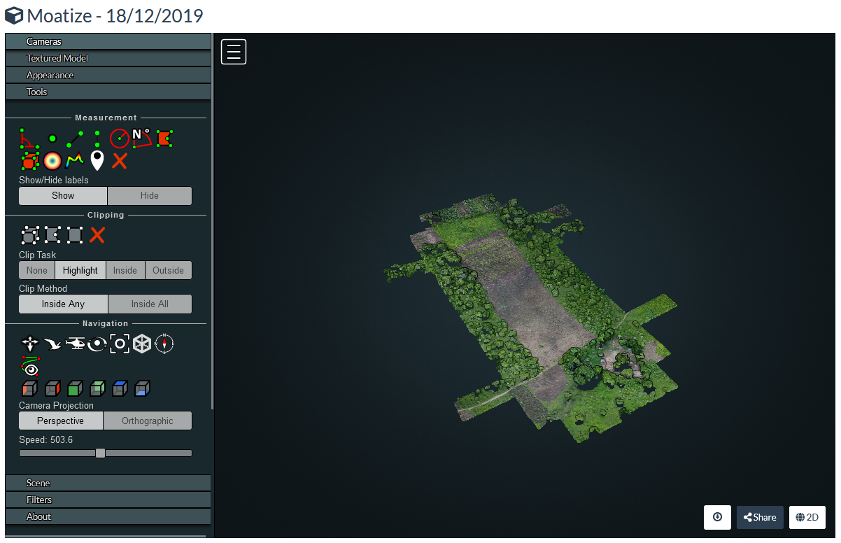
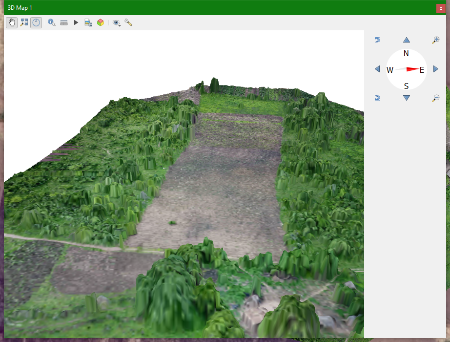
10.1. Features of the 3D View
The 3D View has nice features to visualise the data in 3D.
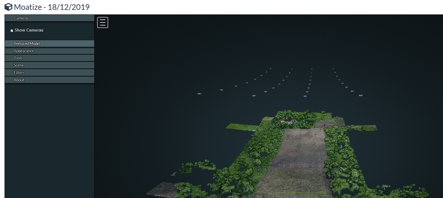
Let's first visualise the position of the camera of the drone when the images were taken.
1. Under Cameras check the box Show Cameras and inspect the result
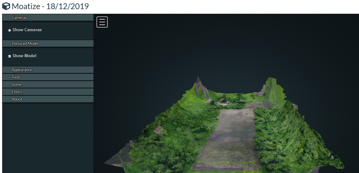
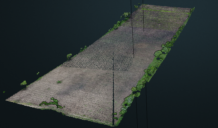
We can also visualise texture instead of the point cloud with the RGB colours.
2. Switch off the cameras.
3. Under Textured Model check the box Show Model.
This will take a little time to show up.
4. Check the result. What do you observe at the boundaries of the image?
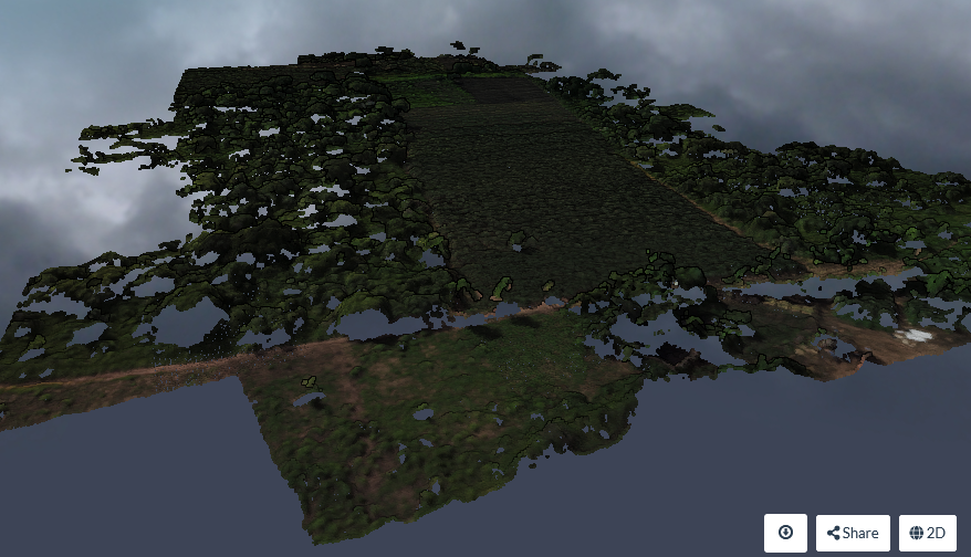
We can also change the appearance of the point cloud.
5. Uncheck the Show Model under Textured Model, so we can see the point cloud again.
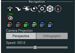
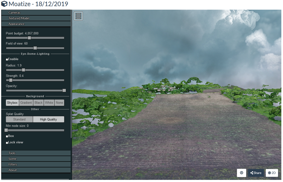
6. Under Appearance you can play with different settings, such as:
- Point budget: the amount of points to visualise
- Field of view determines how much of the scene is visible from our point of view
- You can disable Eye-Dome-Lighting to see the points without shading effect
- Change the background to Skybox to get a dramatic sky over the scene
In the next section we'll explore measurements in the 3D View.
10.2. Measurements in the 3D View
The 3D View comes with a set of measurement tools.
1. Expand the Tools section.
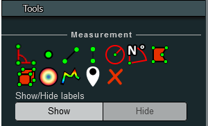
You can explore these tools for different measurements in the 3D space:
 Measure angles between different 3D points you select in the scene
 Point measurement: returns the x, y and z coordinate of a selected location
 Distance measurement between selected points
 Height measurement: difference in height of two selected points
 Cirkel measurement
 Measure the angle between 2 points in degrees of the compass
 Measure areas of polygons
 Measure volumes
 Measure volumes
 Draw a height profile
 Add annotations
 Remove all measurements
2. Try these tools to do measurements in the 3D View.
In the next section we're going to clip areas.
10.3. Clipping
Sometimes we're not interested in the entire scene. In our case we're only interested in the field of interest. There are different clipping tools available.
1. Expand the Clipping section.
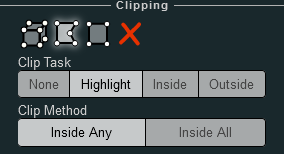
The different methods are:
 Clip a volume
 Clip a polygon
 Draw a selection box. For this method you need to switch to Orthographic view under Navigation.
Under Clip Task you can indicate if you want to Highlight the points inside the polygon, show the points only Inside the polygon or show only points Outside the polygon.
2. Use this a tool to show only the points inside the maize field of our interest.
In the next chapter we'll export the data so we can use it in GIS.
11. Download Assets
Although WebODM has some nice tools for visualising data and to do measurements, you might want to do further processing in GIS.
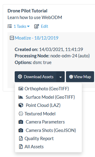
You can download the data (assets) from different places in WebODM:
- If you're still in the 3D View you can click on
 in the lower right of the window.
 - If you're in the Dashboard you can click on Download Assets
12. Use the results in QGIS
Now we have downloaded the data from WebODM, we can visualise and process the results in QGIS.
In the next sections you'll:
- Load the layers in QGIS and compare it with satellite images
- Visualise the DSM in 2D and 3D
12.1. View results in QGIS in 2D
Let's visualise our orthophoto and Digital Surface Model in QGIS.
1. Start QGIS Desktop
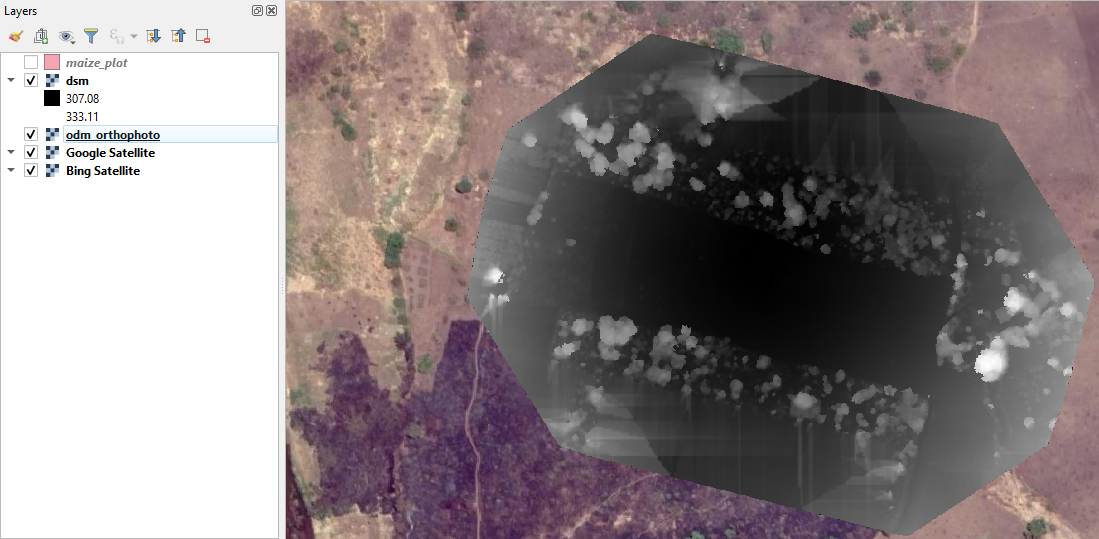
2. Add odm_orthophoto.tif, dsm.tif and maize_plot.shp to the map canvas
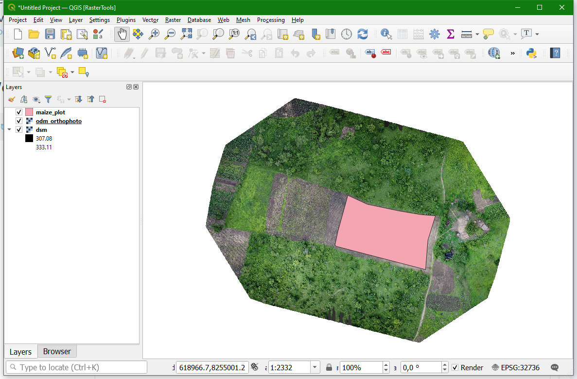
Let's also add a backdrop to see more context around our study area. We're going to install the QuickMapServices plugin.
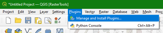
3. In the main menu go to Plugins | Manage and Install Plugins...
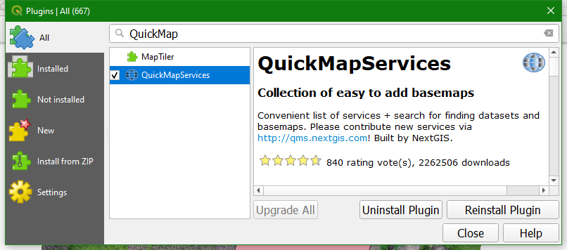
4. Install the QuickMapServices Plugin
5. In the main menu go to Web | QuickMapServices | Settings
6. Go to the More services tab
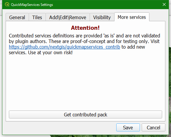
7. Click Get contributed pack
8. Click Save
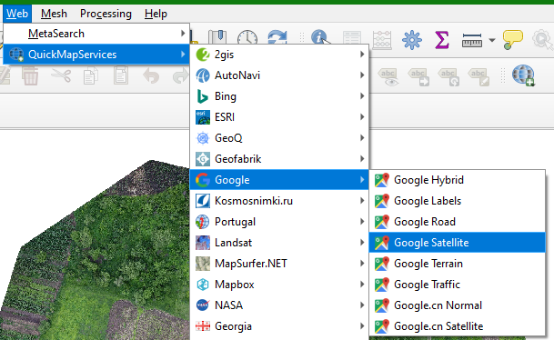
9. In the main menu go to Web | QuickMapServices | Google | Google Satellite
10. In the same way also add the Bing Satellite layer and compare the orthophoto with both satellite images.
- What is the projection of the products created in WebODM?
- What is the spatial resolution of the products?
12.2. View results in QGIS in 3D
Let's have a closer look at the DSM.
1. Make sure we can see the DSM by moving it to the top and/or switching off the other layers.
2. Select the dsm layer in the Layers panel and click  to open the Layer Styling panel.
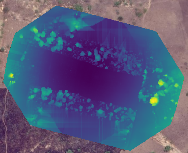
3. Choose the Singleband pseudocolor renderer and style the layer with the Viridis colour ramp.
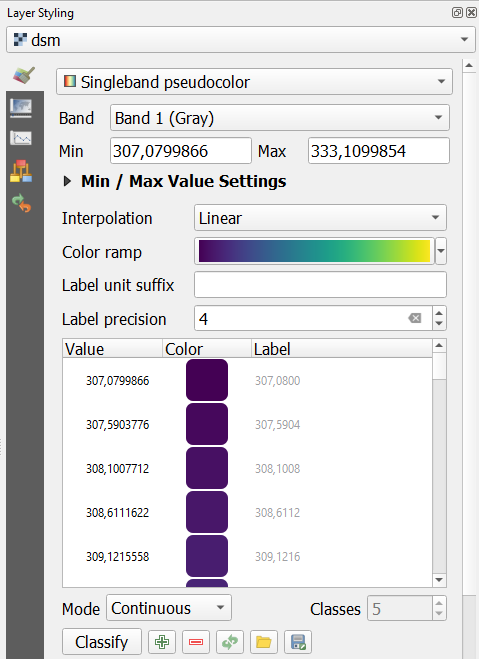
The result now looks like the screenshot below:
Let's now visualise the elevation in the QGIS 3D View.
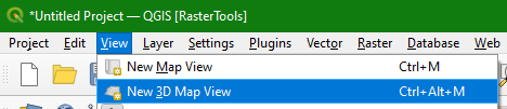
4. In the main menu choose View | New 3D Map View
5. Click on  to go to the settings.
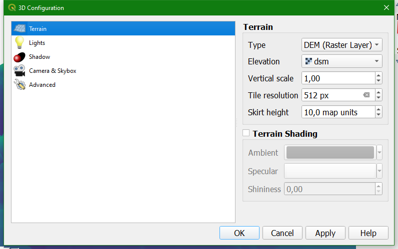
6. Fill in the dialogue as the screenshot below and click OK.
Now you'll see the scene in 3D:
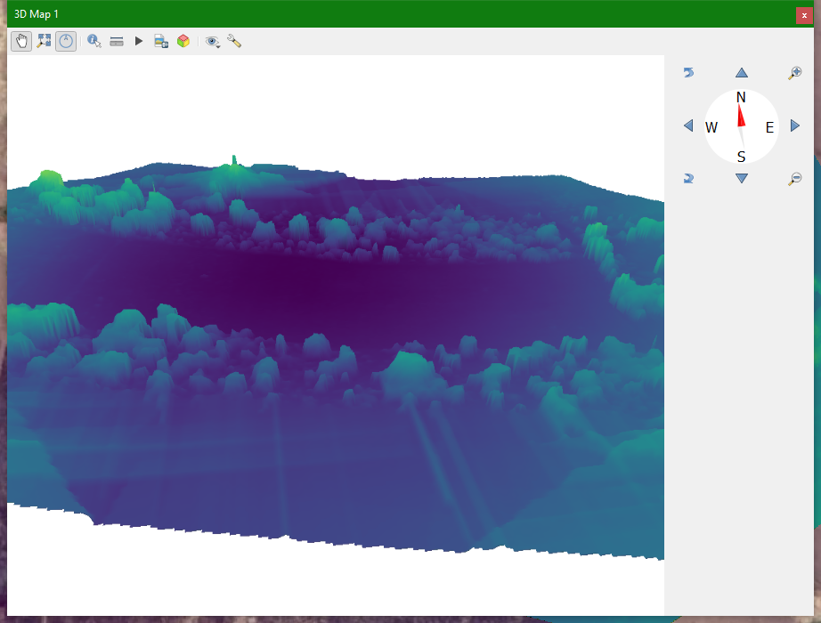
7. Enable the orthophoto in the Layers panel and the 3D View will update so you can see the orthophoto in 3D.
8. Save the QGIS project. We're now going to process the images of 2020. Later we'll compare the results here in QGIS.
13. Process the images of 2020
Now repeat the procedure to derive the orthophoto and DSM for the images of 2020 which you can download here: Moatize_Flight_20200122.tar.gz
- Describe the differences that you observe.
14. Compare results in QGIS
Now we've processed the images of 2019 and of 2020 we can compare the results in QGIS.
1. Start QGIS Desktop
2. Open the project that you have saved in section 12.2
3. Add the DSM and orthophoto of 2020 to the project
4. Compare the 2 orthophotos and DSM's.
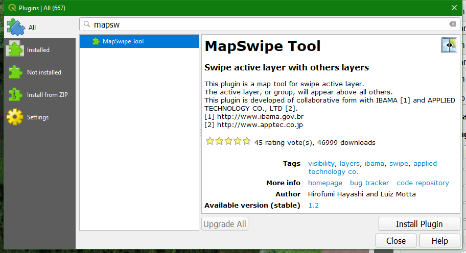
To make the comparison easier, we're going to install the MapSwipe Tool plugin.
5. In the main menu go to Plugins | Manage and install plugins...
6. Install the MapSwipe Tool plugin
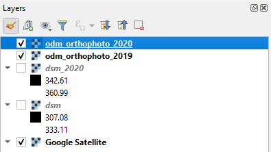
7. Make sure that the orthophotos are on top of the layers list. You can rename them in such a way that you can see to which year they belong.
8. Select the orthophoto of 2020
9. Click on the  icon in the toolbar to activate the MapSwipe Tool plugin.
10. Click in the map canvas and drag the mouse from left to right or from up to down.
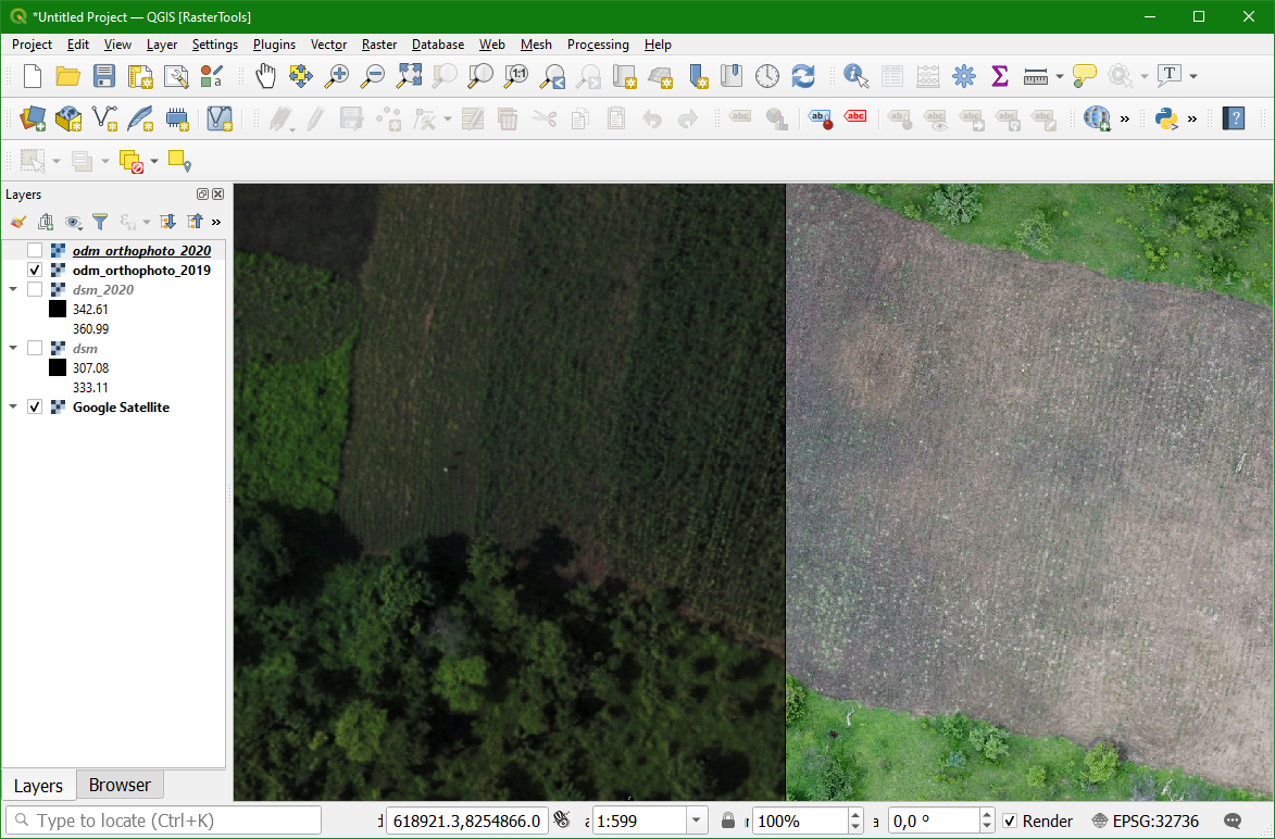
- Describe the differences