Tutorial Zonal Statistics and Area Computations
| Site: | OpenCourseWare for GIS |
| Course: | QGIS Advanced Tutorials |
| Book: | Tutorial Zonal Statistics and Area Computations |
| Printed by: | Guest user |
| Date: | Monday, 27 July 2026, 1:48 PM |
1. Introduction
After this lesson you will be able to:
- calculate zonal statistics from a continuous raster layer using areas defined by a polygon vector layer
- calculate zonal statistics from a continuous raster layer using zones in a discrete raster layer
- calculate the surface area of classes in a discrete raster
- calculate the surface area of classes in a discrete raster per area defined by a polygon vector layer
- calculate other univariate statistics from raster layers
In this lesson we will use the following data that is provided as a GeoPackage from the main module page:
- subcatchment layer with polygons delineated from the DEM
- DEM raster derived from the SRTM 1-Arc Second product. Downloaded from USGS Earth Explorer and further processed in QGIS.
- CORINE 2018 Land Cover 100 m raster provided by Copernicus
- NDVI derived from a Sentinel 2 image of 7 May 2020. Downloaded from USGS Earth Explorer and further processed in QGIS.
2. Theory
Watch this video on the GIS Raster Data Model.
3. Data exploration
Let's first start QGIS.
1. Start QGIS Desktop with GRASS. We'll need GRASS in Chapter 6 of this tutorial.
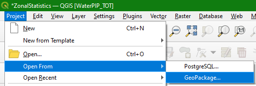
2. In the main menu choose Project | Open From | GeoPackage...
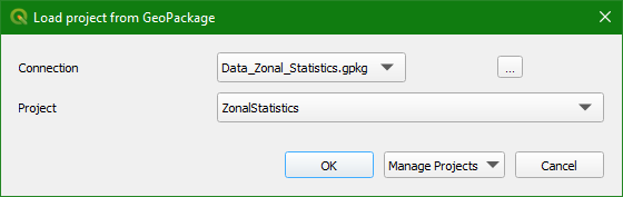
3. In the Load project from GeoPackage dialogue use the  button to browse to the provided Data_Zonal_Statistics.gpkg file, choose the ZonalStatics project and click OK.
Now let's explore the data.
4. Click right on subcatchments and choose Properties.
5. Go to the Information tab and check the metadata.
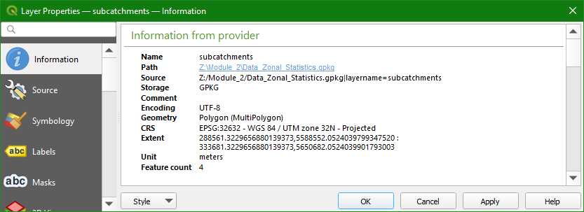
- Does the data contain points, lines or polygons?
- Where is the data stored?
- What is the projection?
- What are the attributes?
8. Go to the Information tab and check the metadata.
- Is this a raster or vector?
- Where is the data stored?
- What is the projection?
- What is the minumum, maximum and average values?
- What is the cell size?
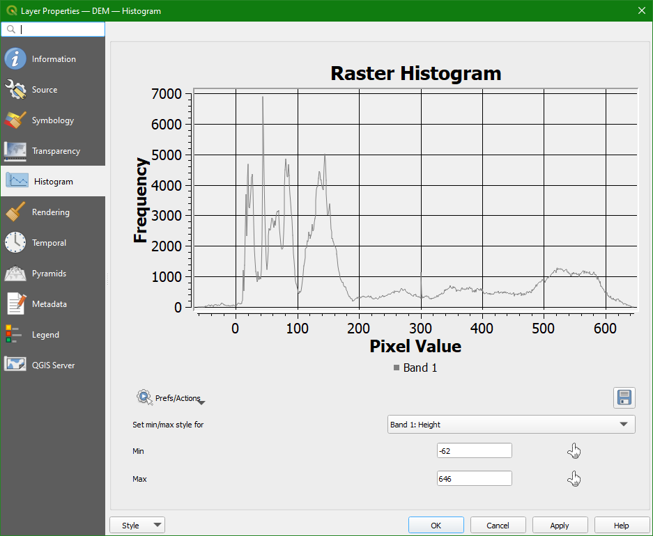
- Describe the distribution of the elevation values.
 to save the plot to a PNG file and check the result
4. Zonal statistics with a raster and a vector layer
Let's first look at how to use a polygon vector layer with zones to extract the statistics from a continuous raster layer.
4.1. Style a continuous raster
Make sure you see the project with layers subcatchment and DEM visible in the map canvas. In this chapter we'll only work with those layers.Let's first style the Digital Elevation Model (DEM) so we can clearer see the value range.
The default legends produced by Desktop GIS software are often not
intuitive, because the software does not know (1) what information is
presented, and (2) the raster data type (e.g. Boolean, discrete or
continuous data). To help interpret the results it is good practice to
style your layers intuitively.
The
DEM is a continuous raster. Continuous rasters represent gradients and
can therefore contain real numbers (or floating point). Continuous
rasters are styled in QGIS using ramps in the Singleband pseudocolor dialogue.
1. Select the DEM layer and click ![]() to open the Layer Styling panel (or press
to open the Layer Styling panel (or press F7).
2. In the Layer Styling panel choose Singleband pseudocolor
from the drop-down list.
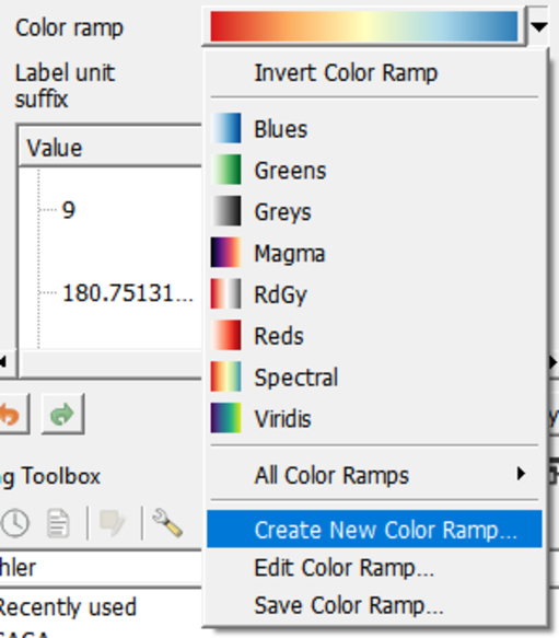
3. Right-click on the color ramp and choose Create New Color Ramp.
4. In the popup Color ramp type dialogue choose Catalog: cpt-city from the drop-down list and click OK.
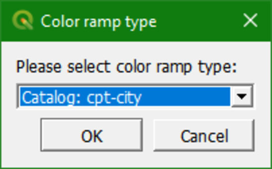
The cpt-city catalogue has a lot of useful preset color ramps.
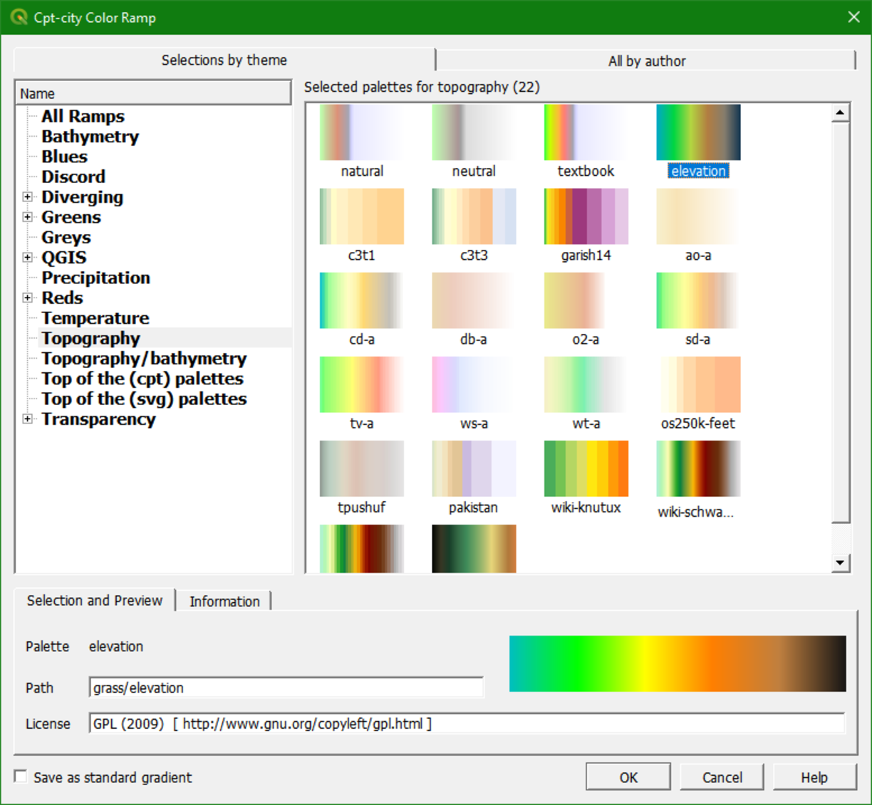
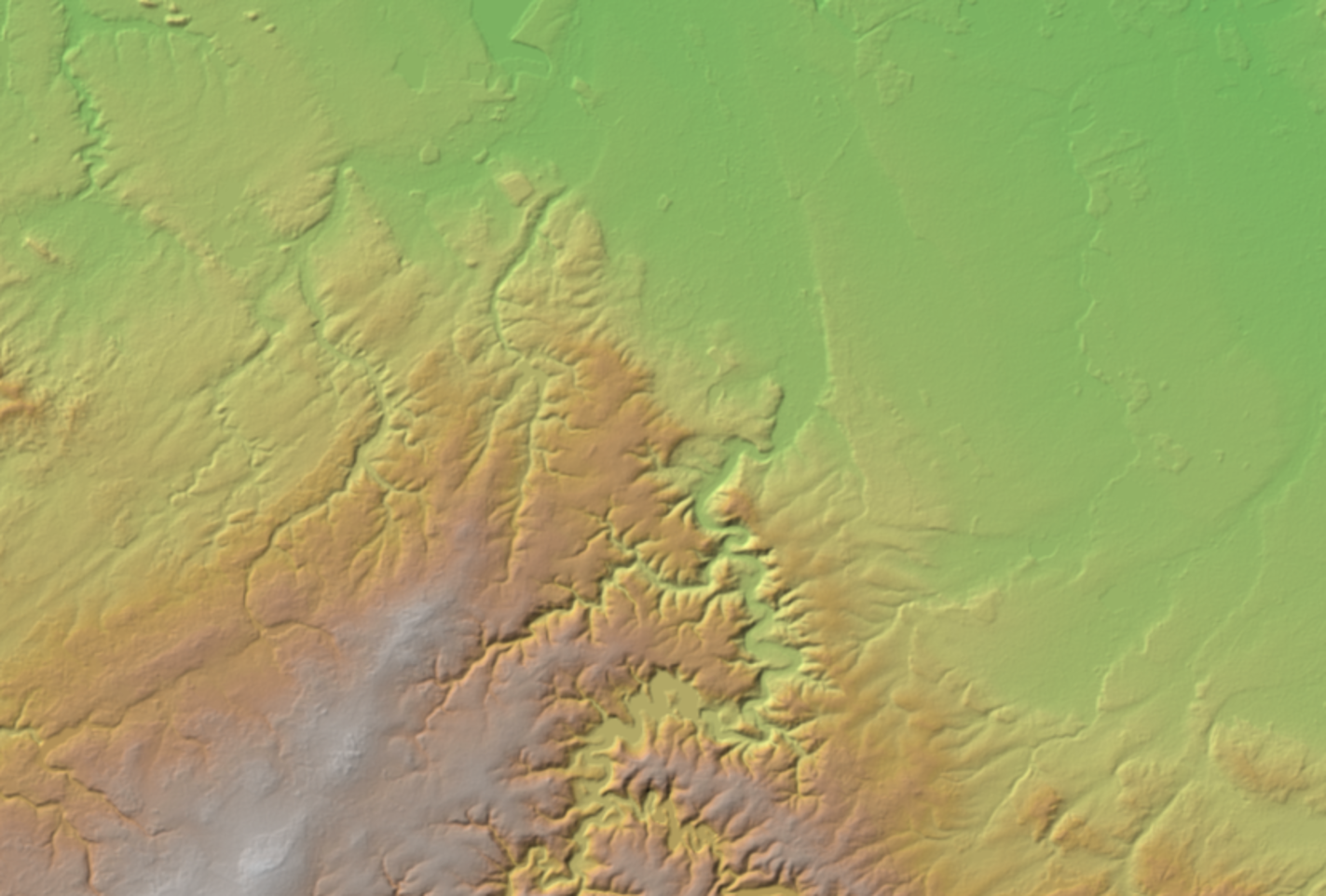
5. Choose Topography | Elevation. Note that cd-a and sd-a are also nice choices. Click Classify in the Layer Styling panel to apply the ramp.
This
gives us more intuitive colors in the DEM where we can clearly
distinguish higher and lower areas. Now we will further improve the
visualisation.
6. Right-click on the DEM layer in the Layers panel and select Duplicate Layer.
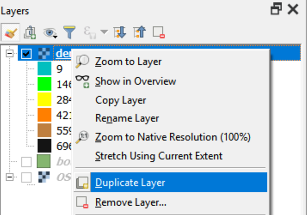
This creates a copy of the DEM layer called DEM copy.
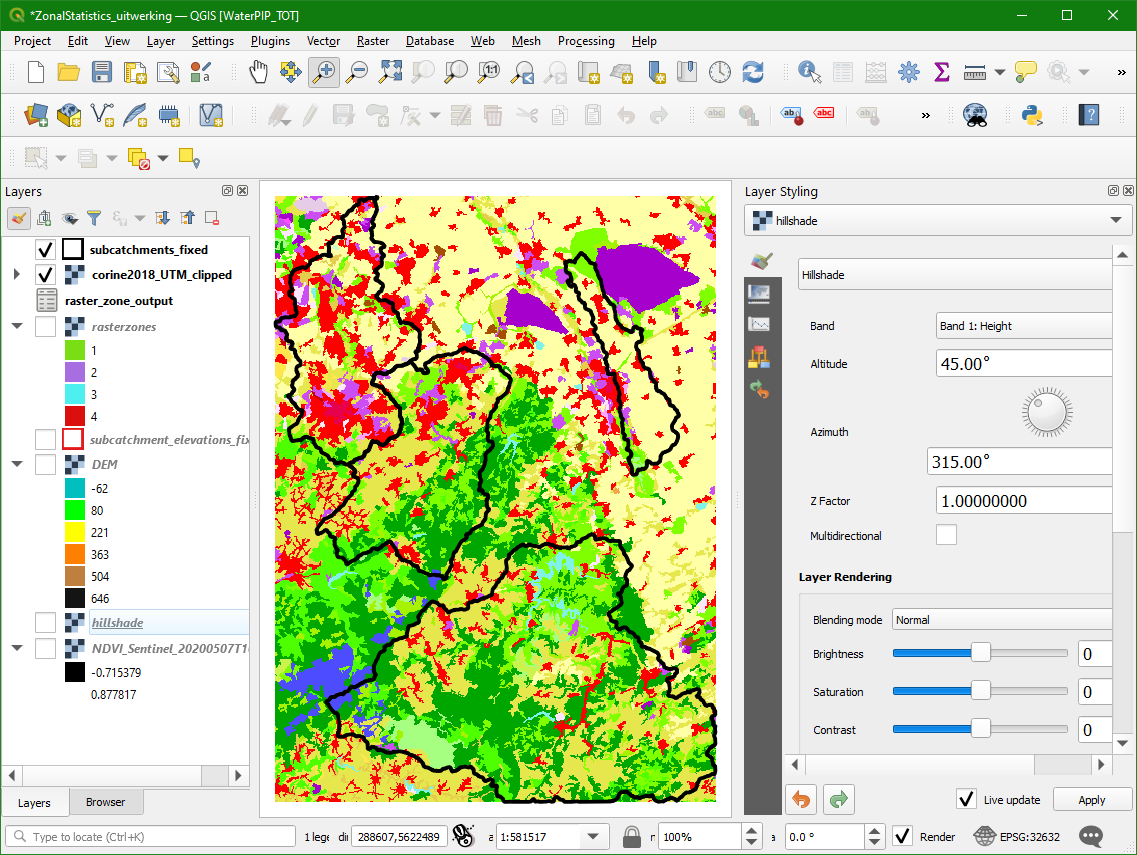
7. Uncheck the DEM layer, check DEM copy and rename the layer to hillshade.
8. In the Layer Styling panel, which should still be open, make sure that the hillshade layer is now selected. In the drop-down list change Singleband pseudocolor to Hillshade.
Now the hillshade layer is visualised with a shading.
Which direction is the illumination coming from? Is this possible in reality?
Hillshade
gives the best results with an artificial illumination in the
northwest, which in reality can not exist in the Northern Hemisphere. If
you move the dial in the Layer Styling panel to the southwest, you will see an inverted relief. Also note that there is a Resampling
section. The default resampling method for both Zoomed in and Zoomed
out is Nearest Neighbor. This method is fine for categorical data
however, elevation is considered continuous data. You should therefore
choose a Zoomed in resampling method of Bilinear and a Zoomed out resampling method of Cubic.
Next, we're going to blend the DEM with the hillshade layer.
9. Switch on the DEM layer by checking the box.
10. In the Layer Styling panel make sure the dem_fill layer is selected. In the Layer Rendering block of the panel, change the Blending mode to Multiply.
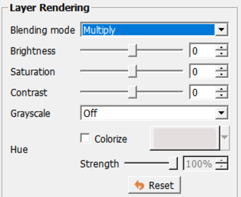
As
you can see, blending gives a much nicer effect than transparency. With
transparency the colours will fade. Now we can clearly see the elevation
differences: the gradient from south to north and the valleys where we
expect the streams.
4.2. Calculate zonal statistics
In this section we'll use a tool from the Processing Toolbox to calculate the zonal statics from the DEM using the subcatchment polygons. The Processing Toolbox
in QGIS provides a lot of tools for processing GIS data. Besides QGIS
tools, it also has tools from GDAL, GRASS, and SAGA that are very
useful.
1. You can activate the Processing Toolbox by choosing Processing | Toolbox from the main menu.
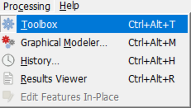
Now the Processing Toolbox panel shows up.
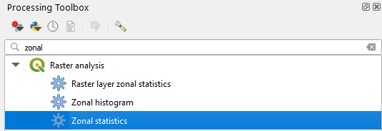
2. In the Processing Toolbox click on Raster analysis | Zonal statistics (you can use the search box to search for it)
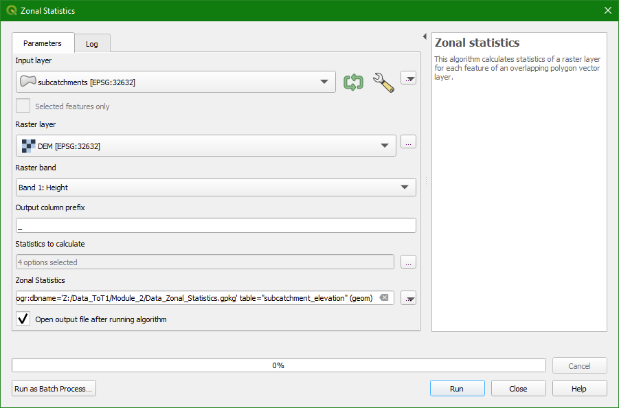
3. In the dialogue choose subcatchments as Input layer and DEM as Raster layer. We leave the Output column prefix as default.
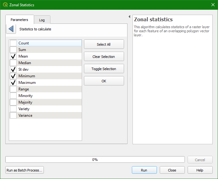
4. Click on  to choose the statistics that you want to calculate. Here choose Mean, St dev, Minimum and Maximum and click OK to return.
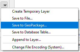
5. At the Zonal Statistics field use the dropdown menu to choose Save to GeoPackage. There browse to the GeoPackage of this project and indicate in the popup that you want to use subcatchment_elevation as the layer name.
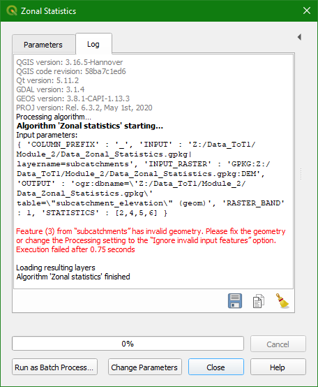
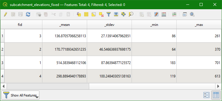
- Which subcatchment has the highest average elevation?
- Which subcatchment has the lowest elevation?
- Which subcatchment has the highest variability in elevation?
5. Zonal statistics with two raster layers
In this chapter we're going to do the same as in the previous chapter. However, instead of using a polygon layer, we'll use a discrete raster layer with zones to derive the zonal statistics for the DEM.
We'll start with styling a discrete raster in the next subsection.
5.1. Style a discrete raster layer
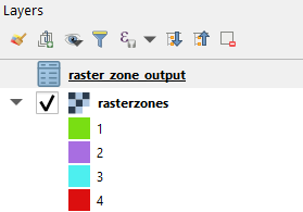
Instead of the subcatchments layer we'll now use the rasterzones layer, which is also provided in the GeoPackage.
The rasterzones layer is a discrete raster where cells have a unique value for the subcatchment they belong to.
1. Make the rasterzones layer visible (check the box) and move it to the top of the Layers panel. You can easily move a layer to the top: click right on the layer name and choose Move to Top.
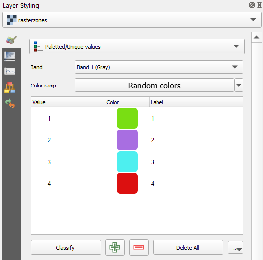
Let's style the rasterzones layer to make more sense out of it. Because it is a discrete raster, we need to use the Paletted/Unique values renderer, which will give each integer cell value a colour.
2. Select the rasterzones layer in the Layers panel and click  to open the Layer Styling panel.
3. Choose Paletted/Unique values as the renderer.
4. To assign random colours to the classes in the raster, click Classify.
Now we're ready to calculate the zonal statistics.
5.2. Raster layer zonal statistics
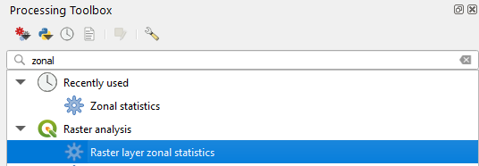
We're going to use another tool from the Processing Toolbox, called the Raster layer zonal statistics tool.
1. Go to the Processing Toolbox and look for Raster analysis | Raster layer zonal statistics.
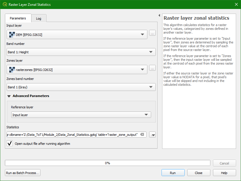
2. In the Raster Layer Zonal Statistics dialogue choose DEM as Input layer from which we want to calculate the statistics. Choose rasterzones as the Zones layer with the classes that we want the statistics for. Under Advanced you can choose if you want to use the Input layer or the Zones layer as the Reference layer for the centroids of the pixels used for the sampling. In our case we can keep it on Input layer. Note that if either the Input layer or the Zones layer has NODATA pixels, these will not be included in the statistics calculations. Save the Statistics layer to the GeoPackage with the layer name raster_zone_output and click Run.
3. Click Close to close the dialogue.
The result is a non-spatial table that has been added to the Layers panel.
Let's check the contents.
4. Click right on raster_zone_ouput in the Layers panel and choose Open Attribute Table.
- Which statistics are reported by the tool?
- Are the values the same as with the Zonal statistics tool that we have used before?
6. Area computations with discrete rasters
For discrete rasters we can calculate the areas using two different tools, which we'll use in the next sections:
- Raster layer unique values report tool
- Zonal histogram
6.1. Raster layer unique values report
Let's first reorganise our layers so we can work on the ones that we need for this part of the tutorial.
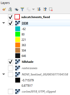
1. Move the subcatchments_fixed layer to the top and move the corine2018_UTM_clipped layer to the second position from the top.
2. Change the line colour of the subcatchments_fixed layer to black to make it more visible. Hide the other layers below.
Your screen should now look like this.
Now we're ready for the area analysis.
3. In the Processing Toolbox choose Raster analysis | Raster layer unique values report.

4. In the dialogue choose corine2018_UTM_clipped as Input layer.
5. We can generate a report in HTML format and/or as a table. Let's try both options. Save the Unique values report to report.html and save the Unique values table to our GeoPackage with the layer name unique_values.
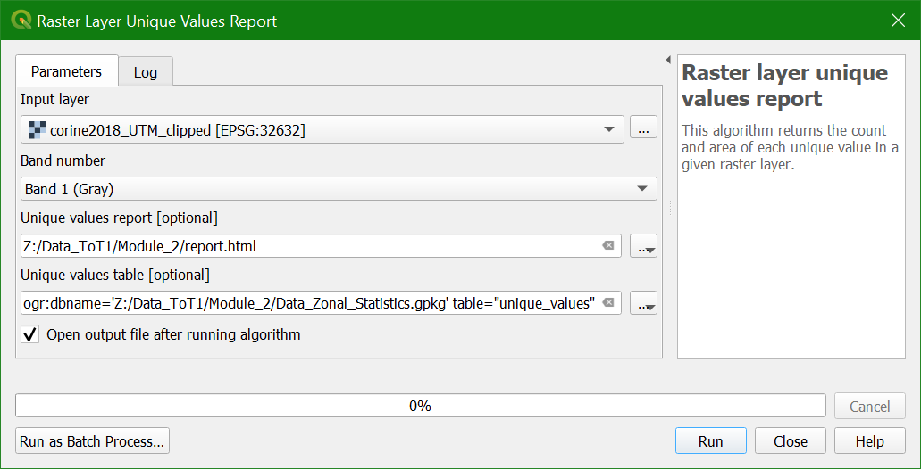
6. Click Run and Close the window after processing.
You can find the HTML results in the Results viewer panel:
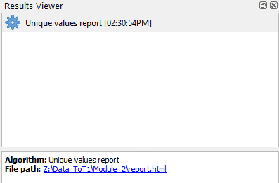
7. You can click on the item or open the html file. Check the result.
8. Now open the unique_values table that was added to the Layers panel (click right and choose Open Attribute Table).
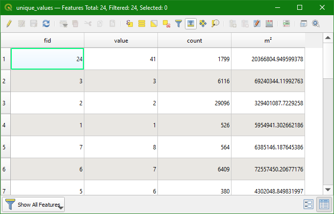
You can see that it gives for each class in the raster layer the count (nr. of pixels) and the area in m2.
In the next subsection we're going to calculate the are per subcatchment.
6.2. Zonal histogram
In the previous subsection we have derived the areas of all classes in the land cover map for the entire raster layer. However, we are more interested in the class area per subcatchment. We can calculate that with the Zonal histogram tool.
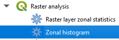
1. In the Processing Toolbox look for Raster analysis | Zonal histogram.
2. In the Zonal Histogram dialogue choose corine2018_UTM_clipped as Raster layer and subcatchments_fixed as Vector layer containing zones. Save the Output zones to the GeoPackage with the name zonal_histogram and click Run.
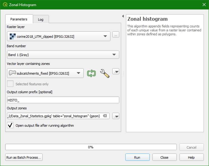
3. Click Close to close the dialogue.
4. In the Layers panel move the new zonal_histogram layer to the top and copy the style from the subcatchments_fixed layer to zonal_histogram.
5. Now open the attribute table of zonal_histogram and inspect the results.
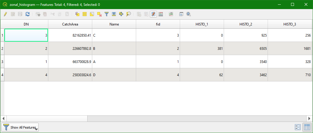
You can see that the features are the four subcatchments and that in the HISTO_# fields we have the number of pixels in each class.
- How can we calculate the surface area in m2 of each class in each subcatchment?
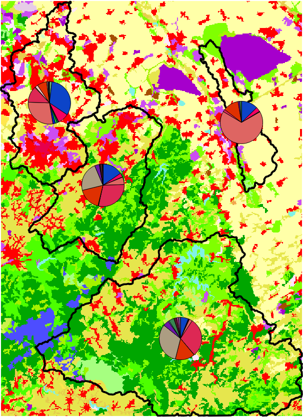
6.3. Visualise with pie charts
A quick way to visualise the results of the previous subsection is to use diagrams.
1. In the Layers panel click right on the zonal_histogram layer and choose Properties...
2. In the Layer Properties window choose the Diagrams tab.
3. Choose Pie Chart from the drop down menu.
4. Select all HISTO fields and click  to add them to Assigned attributes.
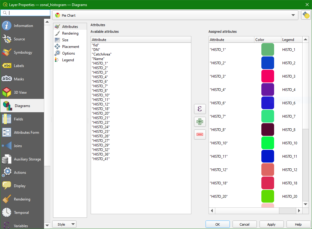
There you can change the colours and the text of the legend.
As you see we have a lot of classes. Here we are using CORINE Level 3 classes. In reality we might want to use the more aggregated Level 1 classes. In QGIS you can reclassify rasters with the Reclassify by table tool in the Processing Toolbox.
5. Click OK to see the result on the map
In the next chapter you'll learn another tool to calculate additional univariate statistics.
7. Calculate additional univariate statistics
Sometimes we're also interested in percentiles. We can calculate these easilty with the r.univar tool from GRASS which is available in the Processing Toolbox.
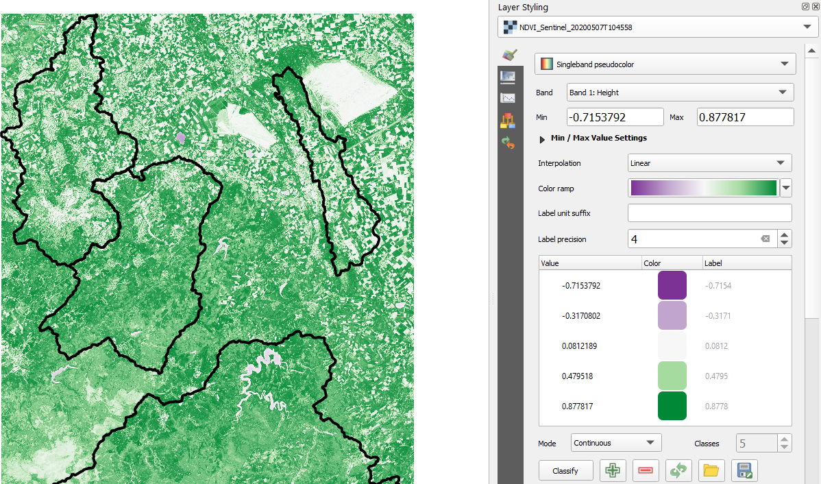
For this chapter we're interested in the statistics for the NDVI raster. NDVI is the Normalized Difference Vegetation Index, which is derived from satellite data to detect green vegetation cover. It has values from -1 to 1, where values larger than 0 represent vegetation cover.
NDVI in this tutorial was derived from a Sentinel 2 image of 7 May 2020 and has a spatial resolution of 10 m.
Let's first style the NDVI layer.
1. Move the NDVI_Sentinel_20200507T104558 layer to below the subcatchments_fixed layer and make sure it's visible.
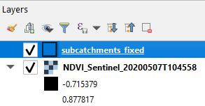
2. Select the NDVI_Sentinel_20200507T104558 layer and click  to open the Layer Styling panel.
- What raster data type is NDVI? What renderer should we use for styling?
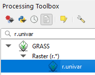
4. In the Processing Toolbox look for GRASS | Raster (r.*) | r.univar.
Note that if you can't use the GRASS tools, you need to start QGIS Desktop with GRASS as mentioned at the start of this tutorial. Only then you can use the GRASS tools in the Processing Toolbox.
5. In the r.univar dialogue make sure to set the following input:
- The NDVI_Sentinel_20200507T104558 layer should be selected as Name of raster map(s)
- Select rasterzones as Raster map used for zoning. Note that you can only have a raster with zones. It will not work with polygones.
- For Percentile to calculate type
5,99. In this way the 5th and 99th percentile will be calculated. Percentiles need to be separated by comma. - For field separator type
comma. This will be the column separator that will be used in the output text file. - Because we want to calculate the indicated percentiles we have to check Calculate extended statistics in the Advanced Parameters section.
- Write the Univariate results to a text file with the name univar_NDVI_subcatchments.txt.
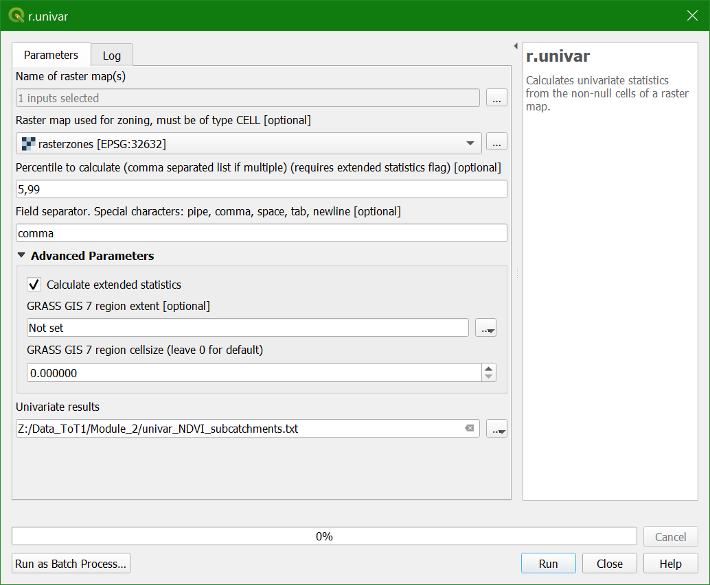
6. Click Run. Click Close after processing.
You can open the text file as comma separated file in a spreadsheet programme. Here we'll add it to our QGIS project.
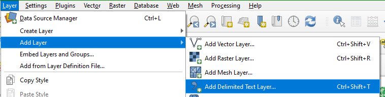
7. In the main menu go to Layer | Add Layer | Add Delimeted Text Layer...
8. In the dialogue browse to the text file. Make sure that CSV (comma separated values) is chosen under File Format. And because our table is non-spatial we need to indicate that under Geometry Definition by selecting No geometry (attribute table only).
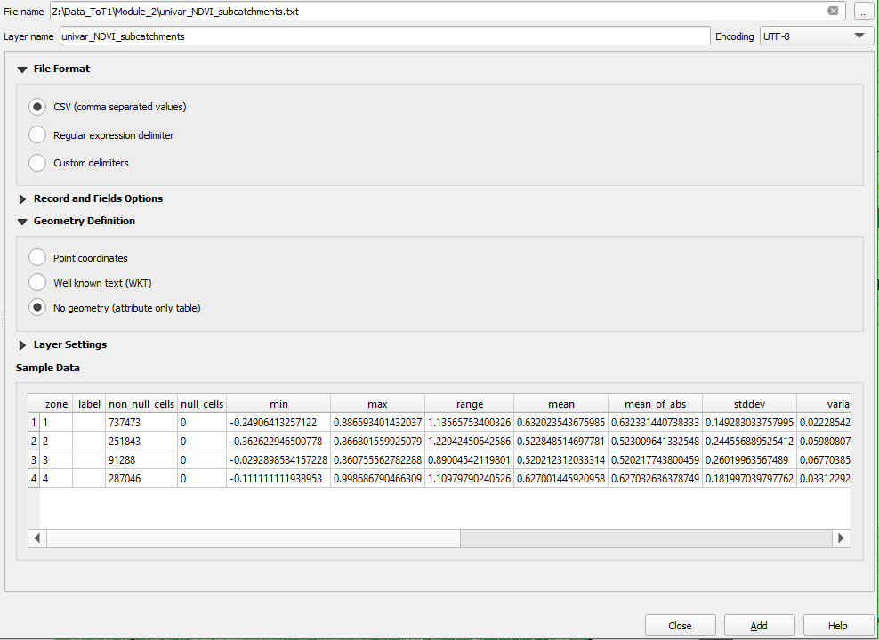
9. If the preview under Sample Data looks good, click Add to add the table to the Layers panel and click Close to close the dialogue.
10. Open the attribute table and interpret the results.
11. Repeat the procedure to get the NDVI statistics per land-cover class.
8. Conclusion
In this tutorial you have learned to:
- calculate zonal statistics from a continuous raster layer using areas defined by a polygon vector layer
- calculate zonal statistics from a continuous raster layer using zones in a discrete raster layer
- calculate the surface area of classes in a discrete raster
- calculate the surface area of classes in a discrete raster per area defined by a polygon vector layer
- calculate other univariate statistics from raster layers