Tutorial Stream and Catchment Delineation using PCRaster in QGIS
| Site: | OpenCourseWare for GIS |
| Course: | FOSS4G 2022 Workshop Hydrological analysis with PCRaster in QGIS and Python |
| Book: | Tutorial Stream and Catchment Delineation using PCRaster in QGIS |
| Printed by: | Guest user |
| Date: | Wednesday, 10 June 2026, 11:16 PM |
Description
Table of contents
- 1. Introduction
- 2. Theory
- 3. Download DEM Tiles
- 4. Mosaic DEM Tiles
- 5. Reproject DEM
- 6. Create a Subset of the DEM
- 7. Fill Sinks and Calculate Flow Direction
- 8. Delineate Streams
- 9. Define Outflow Point
- 10. Delineate the Catchment
- 11. Clipping layers to the catchment boundary
- 12. Styling the Resulting Catchment Area
- 13. Storing the Data in a GeoPackage
- 14. Conclusions
1. Introduction
One of the most important uses of GIS in hydrology is the delineation of catchments and streams. This lesson presents a generic workflow for stream and catchment delineation for areas where only open data is available. The Shuttle Radar Topography Mission (SRTM) 1 Arc Second DEM will be used. The workflow will be applied to the Rur catchment in Germany.
After this lesson you will be able to:
- find and download SRTM DEM tiles from the EarthExplorer website
- mosaic raster layers into a virtual raster
- reproject rasters
- create subsets of rasters
- fill sinks in a DEM
- calculate and style flow direction raster layers
- calculate Strahler orders
- delineate streams
- delineate catchments
- style layers for visualising catchments
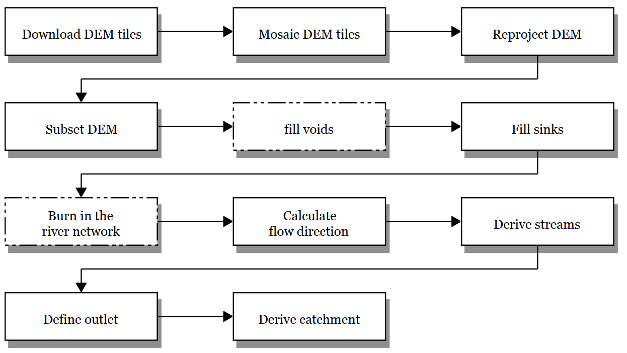
In order to delineate a catchment from a DEM in GIS we need to follow these steps (details covered in this lesson):
1. Download the DEM tiles of your study area. Make sure that the tiles cover at least the study area and that the catchment you want to derive is covered completely. Better to take it a bit larger to avoid boundary effects.
2. If your study area is covered by multiple DEM tiles, you need to mosaic (merge) the tiles to create a single raster DEM layer.
3. The DEM tiles might be in a different coordinate system then desired. In that case you have to reproject the DEM layer to the projection you want to use in the study area.
4. In the case that the merged tiles are much larger than your study area, you can subset (clip) it to a smaller area to reduce calculation time.
5. Interpolate voids when pixels with no data exist in the DEM.
6. Make a hydrologically correct DEM by filling sinks and removing spikes.
7. Calculate the flow direction for each cell.
8. Derive the drainage network.
9. Calculate the catchment for the outflow point of the catchment.
When a map with the stream network already exists, the procedure can be improved by "burning" the river network into the DEM. In that way the DEM is always lower at rivers and runoff will follow the actual river network. This is beyond the scope of this chapter.
The matrials for this lesson can be downloaded from the main lesson page. The next section covers how to download the SRTM tiles from USGS EarthExplorer. These are also included in the course data.
2. Theory
2.1. Digital Elevation Models in GIS
Watch this video on Digital Elevation Models in GIS.
2.2. Stream and Catchment Delineation
Watch this video on the theory of stream and catchment delineation.
3. Download DEM Tiles
For the Rur study area, we will download the tiles from the SRTM 1 Arc-Second global data set. Since the end of 2014 a 1-arc second global digital elevation model (approximately 30 meters at the equator) has been released as open data. Most parts of the world have been covered by this dataset ranging from 54 degrees south to 60 degrees north latitude. A description of the SRTM data products can be found here.
The following steps explain how to download the SRTM DEM tiles for the study area.
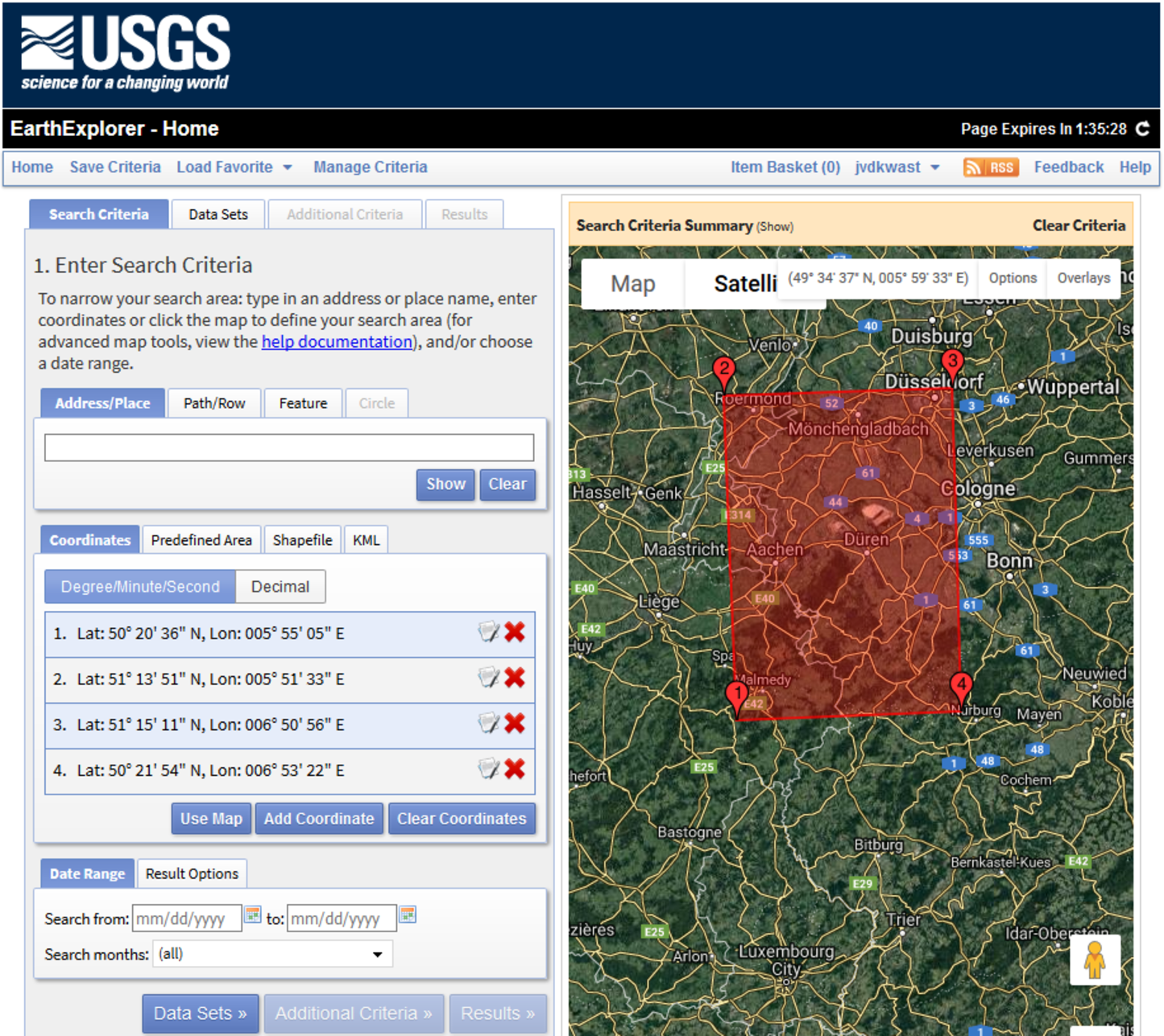
1. Open a browser and browse to http://earthexplorer.usgs.gov
In order to download the SRTM DEM tiles you need to create an account. If you don't succeed with making an account you can use the SRTM tiles provided with the data of this lesson (4 GeoTiff files).
2. Click Register and follow the procedure. After registration, log in to the USGS EarthExplorer portal.
Now we need to indicate the search area. In EarthExplorer this can be done in different ways: (1) Search for a location name, (2) Zoom in on the map and use the coordinates of the zoom area, (3) Upload a KML or zipped shapefile. For this case we prepared a shapefile with a bounding box.
3. Choose Shapefile and upload the boundingbox.zip file (you need to first zip all files belonging to the boundingbox shapefile!).
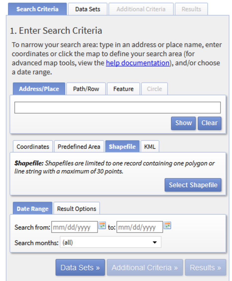
4. Choose Data Sets to go to the next screen where we can select the data set.
5. Click on the plus signs to select Digital Elevation | SRTM | SRTM 1-Arc Second Global. Make sure to tick the box.
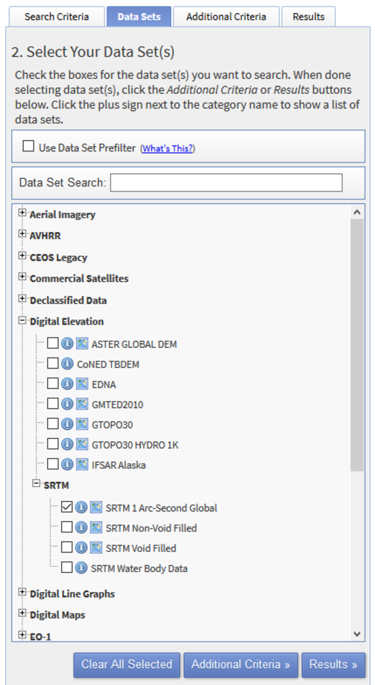
6. Click Results to go to the next screen.
Now you see the search results: four tiles. Before downloading you can check the tiles. With the foot icon, for example, you can see the footprint of the tile.
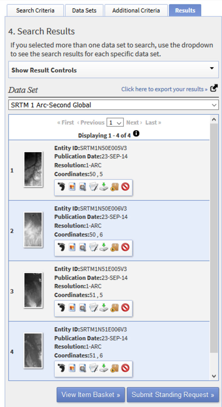
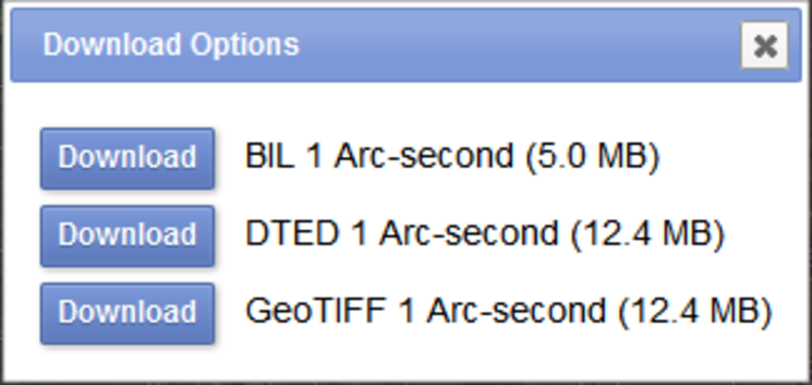
7. Download each tile by clicking the Download Options ![]() button.
button.
8. In the Download Options dialogue download the DEM in GeoTIFF Format to the exercise folder on your hard disk.
The tiles can now be added to your QGIS project.
9. Start QGIS Desktop.
We'll start with a new project.
10. In the Browser panel add the folder with the data for this chapter to the Favorites.
11. Right-click on one of the tiles and choose Properties to review the metadata.
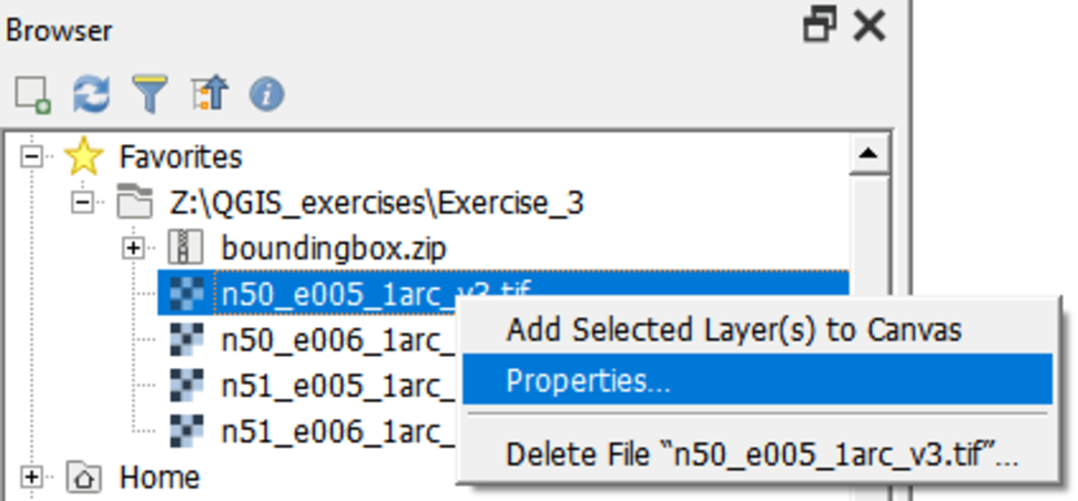
What is the projection? What are the map units?
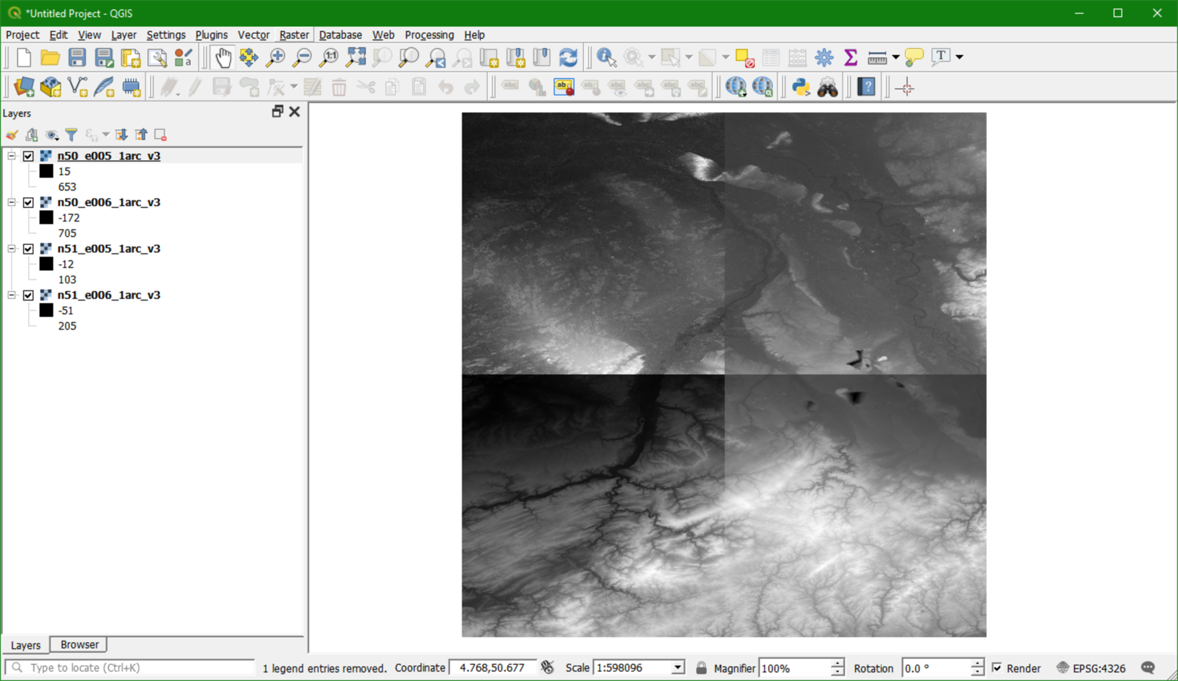
12. Select and drag the four tiles to the Map Canvas.
4. Mosaic DEM Tiles
Before we proceed, we have to merge the four DEM tiles, which in GIS terminology is called mosaic. Here are two ways to mosaic the tiles:
- Merge the tiles into one physical raster file (e.g. GeoTIFF)
- Merge the tiles into a virtual file (.vrt)
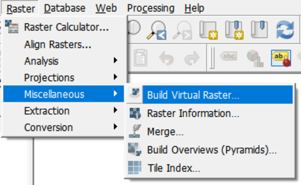
2. In the Build Virtual Raster dialogue you can choose each file individually or merge all files in a directory. We can also merge the files that are visible in the Map Canvas. We'll use the last option:
- At Input layers click
 .
. - Use the Select all button to select the four tiles and click OK (figure
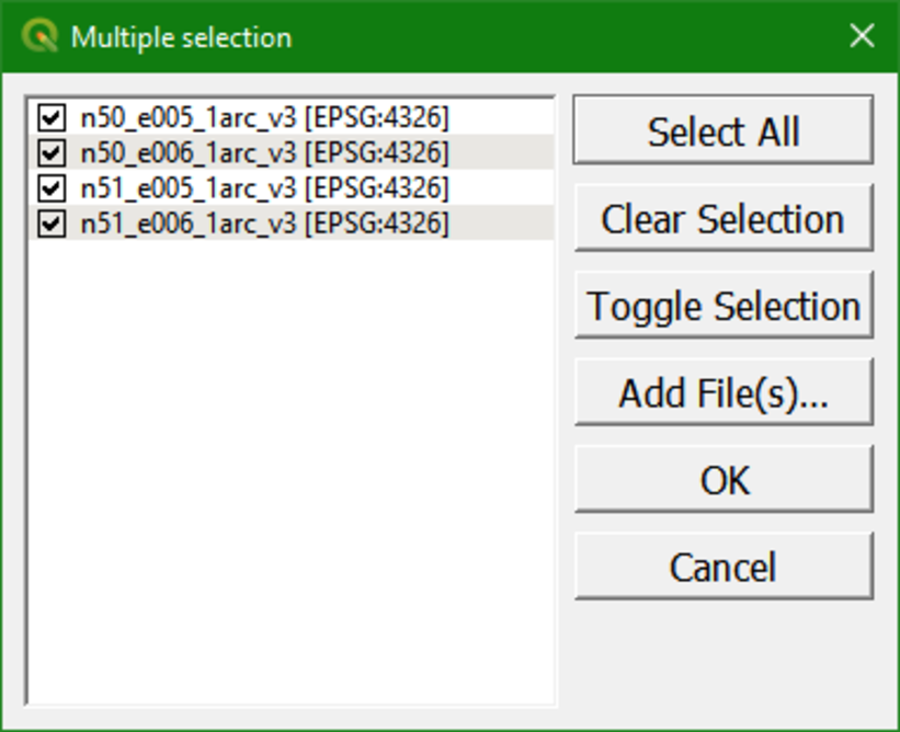
- Browse to the location where you want to save the output file and give it the name
dem_mosaic.vrt.
- By default, Resolution is set to
average. In our case the files all have the same resolution (1 Arc Second).
- Uncheck the box before Place each input file into a separate band. This needs to be checked only if you want to create a mapstack, i.e. with remote sensing bands.
- Keep the Resampling algorithm at the default:
nearest. This also has no impact, because resampling is not needed.
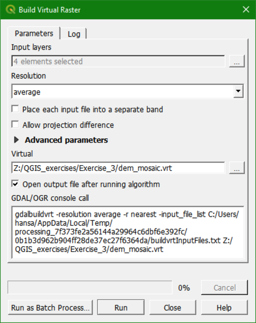
3. Click Run to run the algorithm. Click Close to get back to the main screen where you can see the merged DEM.
You'll notice that in the Map Canvas, the borders of the tiles are not visible anymore in the merged DEM because QGIS stretches the greyscale using the minimum and maximum of the entire merged DEM. This is only for visualisation, the values in the tiles are the same as in the mosaic.
4. Now remove the individual tiles (not the dem_mosaic) from the layers list by selecting them while the
Ctrl button is pressed. Then right-click one of the tile names and select Remove Layer. Click OK to confirm. This will remove the tiles from the screen, but not from the hard disk.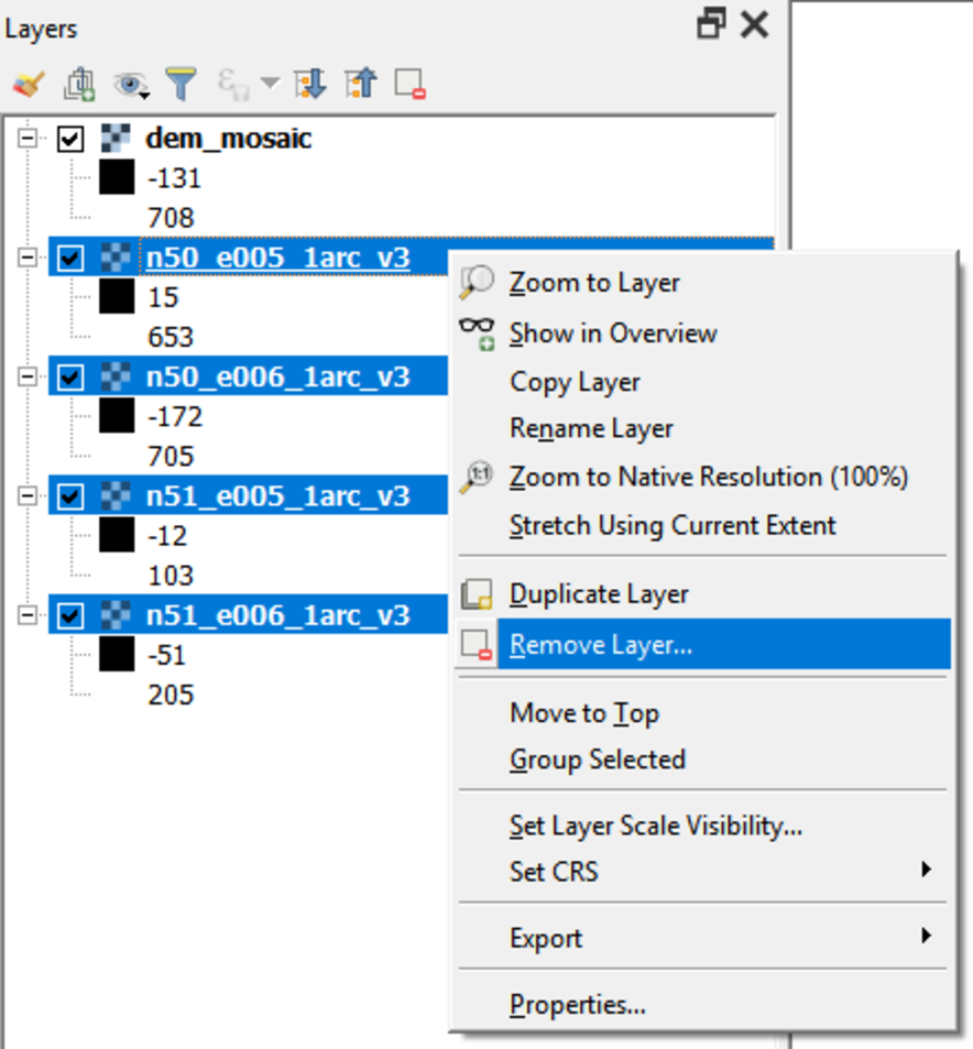
5. Reproject DEM
The DEM is in its original Lat/Lon Geographic Coordinate System (GCS) with datum WGS 84 (EPSG: 4326). It is not recommended to use a GCS for DEM analysis, because the z units (e.g. meters) are different than the x and y units (degrees). We need to choose a projection for our project. If the project covers one country we can choose a national projection. In our case, however, the project covers multiple countries (Germany, the Netherlands, and Belgium). Therefore we will use a global projection: UTM Zone 32 North, with WGS-84 as datum.
We can find the EPSG codes at http://www.spatialreference.org
1. Use the website to search for UTM 32N wgs 84. You can leave QGIS running and open a browser.
The figure below shows the result.
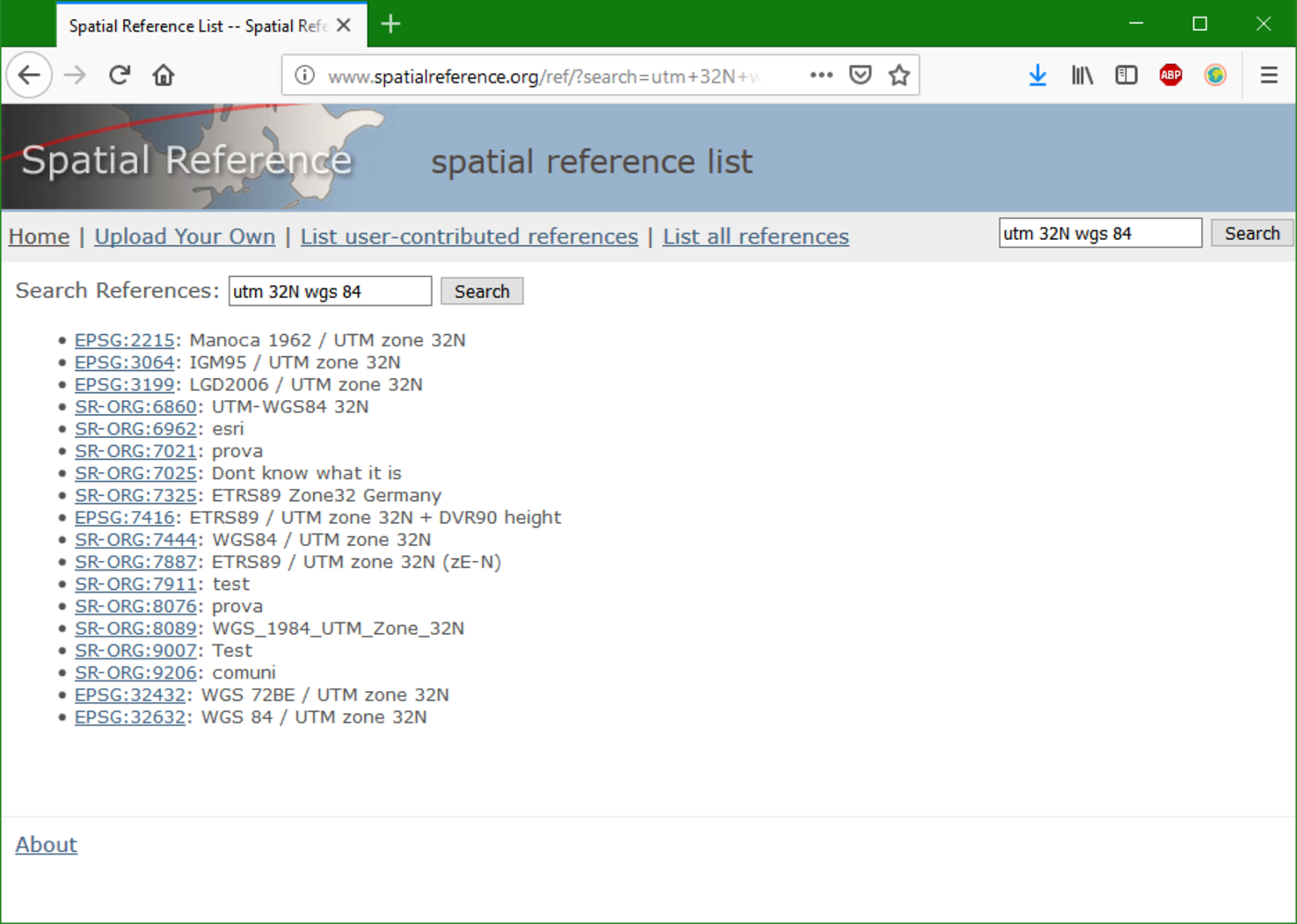
We need to take a look at the EPSG codes. We will use EPSG: 32632 throughout this project - clicking on it will provide more details.
Now we are going to reproject the DEM from unprojected GCS (Lat/Lon WGS 84 - EPSG: 4326) to UTM Zone 32 North / WGS 84 (EPSG: 32632).
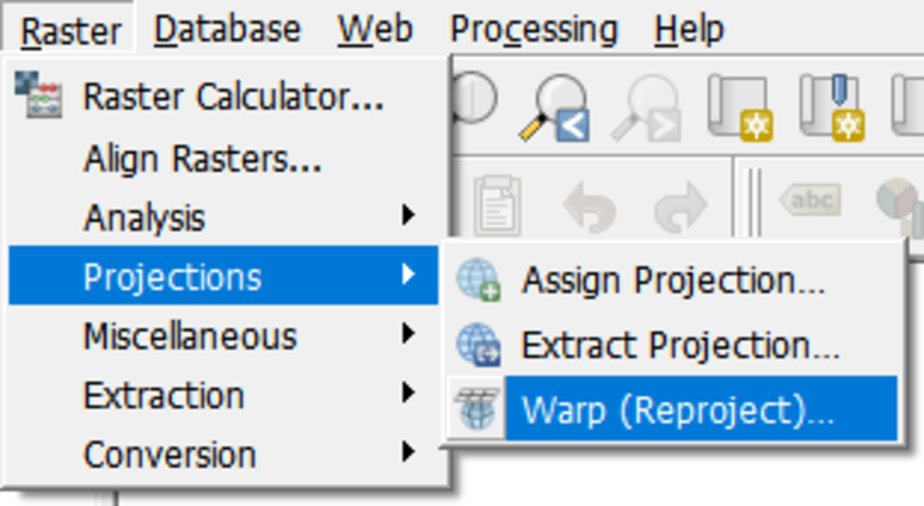
2. From the main menu choose Raster | Projections | Warp (Reproject).
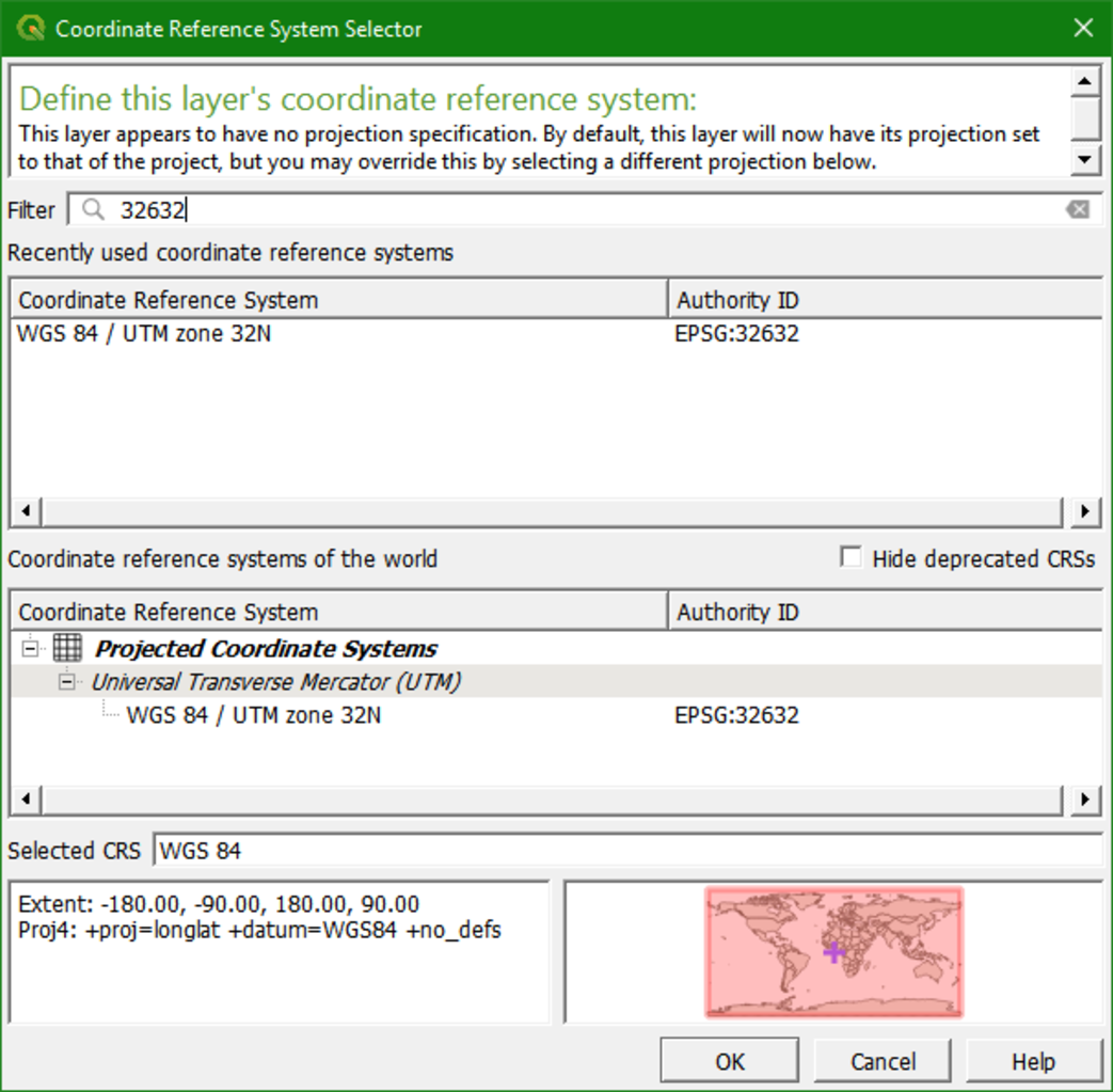
3. In the Warp (reproject) window, click to choose the Target CRS.
4. In the dialogue that opens type 32632 at Filter and select WGS EPSG: 32632 in the middle of the dialogue window and click OK.
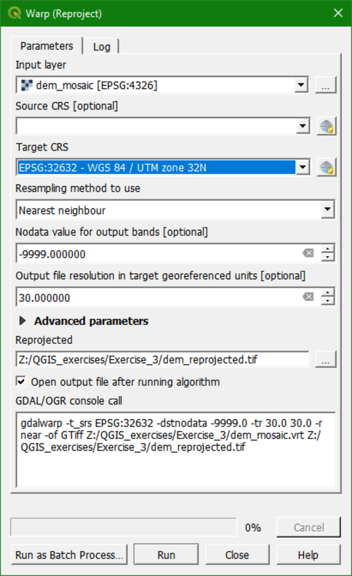
5. Now complete the dialogue:
- For the Resampling method we choose
Nearest Neighborto preserve the elevation values of the original files. - Set the No data value for output bands to
-9999because when the raster layer is reprojected there will be "no data" at the borders. In this way we define that "no data" has a value -9999 and will not be visualised and treated as "data". - Set the Output file resolution to
30m. - Browse to your exercise folder and name the output file
dem_reprojected.tif
The dialog should now look like the figure below.
Note the gdalwarp command that will be executed in the background.
6. Click Run to run the algorithm. After running, click Close to close the window.
The re-projected DEM now appears in the list of Layers. The DEM may seem distorted due to the fact that the Map Canvas Projection is still in Lat/Lon, as indicated by the coordinates in the lower part of the Map Canvas and the EPSG code of the Map Canvas in the lower right corner. This is due to the on-the-fly projection, which causes a difference between the projection in the file and the one that is visualised.
7. To complete this operation, and properly display the new dataset, we need to change the on-the-fly projection of the Project. To do so click on the EPSG:4326 in the lower right of the screen.
![]()
8. In the new dialogue window select the EPSG:32632 projection that is already in the list of Recently used coordinate reference systems, as shown in the figure below , and click OK.
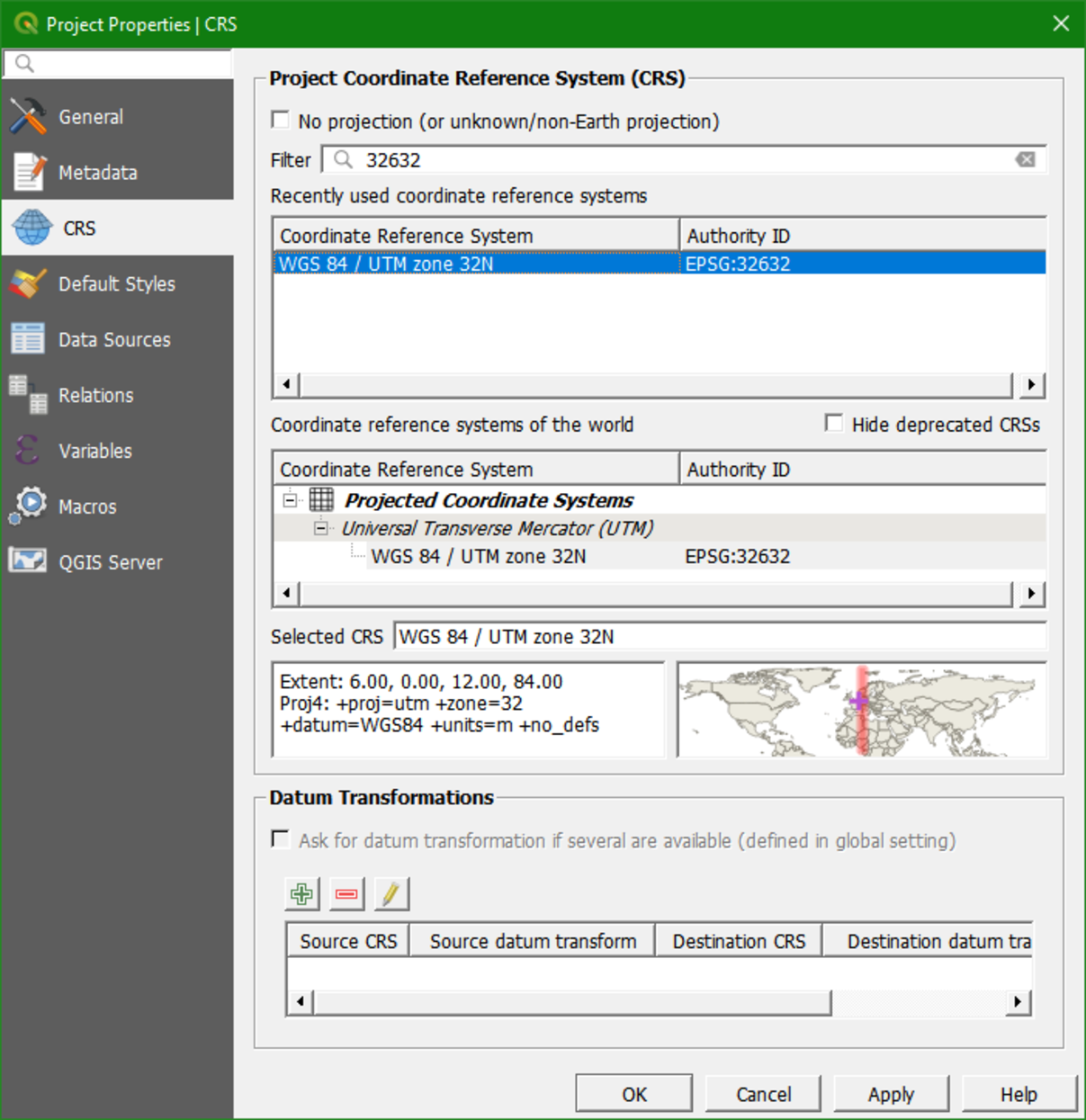
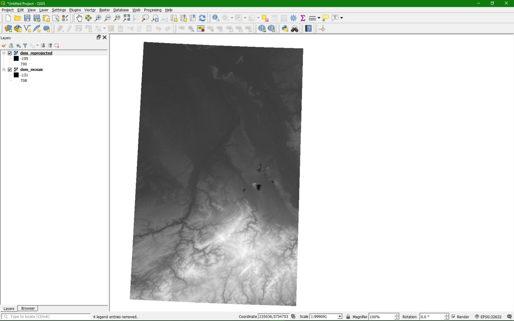
In the Map Canvas the DEM is now displayed in the correct position (with north pointing up), as shown in the figure below. The coordinates of the new display are also in meters as we want.
9. You can now remove the layer dem_mosaic.
This is a good time to save your project.
6. Create a Subset of the DEM
In order to reduce the calculation time of the algorithms, we will subset (or clip) the raster layer. However, it's important to make the boundary of your study area a little bit bigger to prevent boundary effects.
An easy way to select the boundary of your study area is to use OpenStreetMap. OpenStreetMap contains crowd sourced data. If the QuickMapServices plugin is installed, you can add an OpenStreetMap to QGIS as follows:
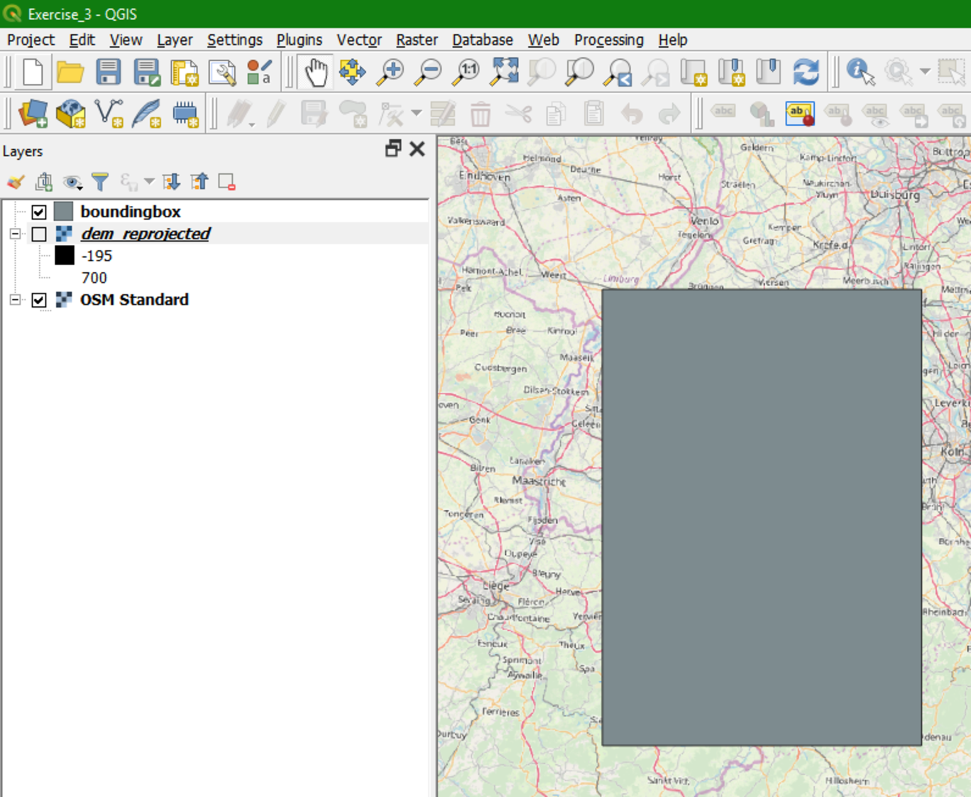
1. In the main menu choose Web | QuickMapServices | OSM | OSM Standard.
2. Now the OpenStreetMap layer will be shown in the Map Canvas. Temporarily hide the DEM by unchecking the box or dragging the OSM layer to the top.
In order to know the approximate extent of the Rur catchment, the exercise data contains a zipped shapefile with the bounding box (the same that we used for downloading the DEM tiles). Note that in reality you'll not have a bounding box, but you should use your expert knowledge to locate the approximate boundaries of the study area.
3. Unzip boundingbox.zip in your exercise folder.
4. Drag the boundingbox.shp layer to the Map Canvas.
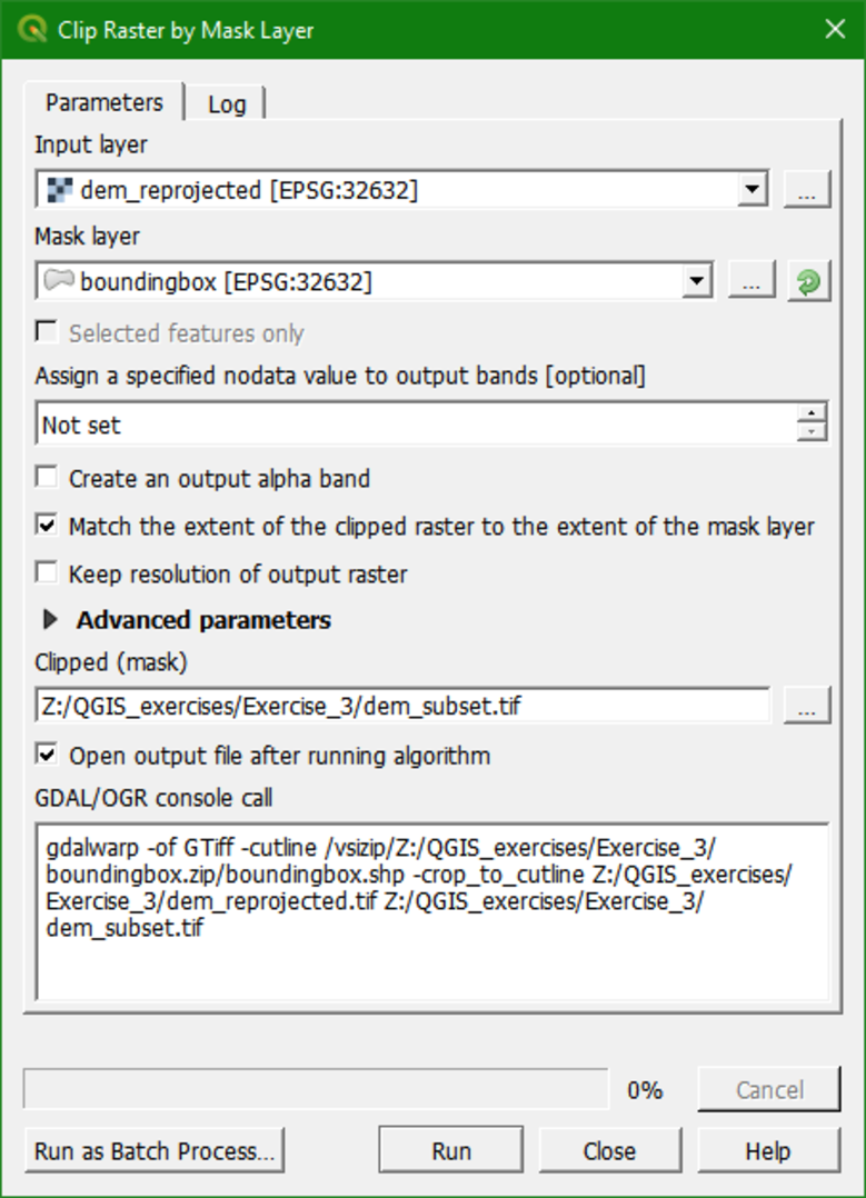
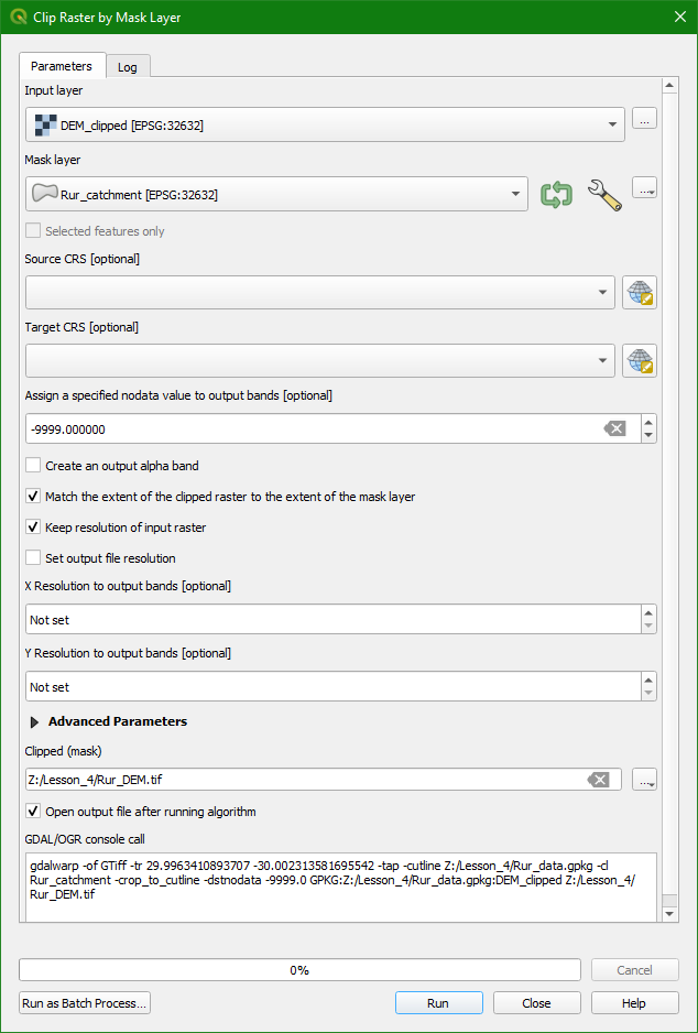
5. Now, from the main menu select Raster | Extraction | Clip Raster by Mask Layer.
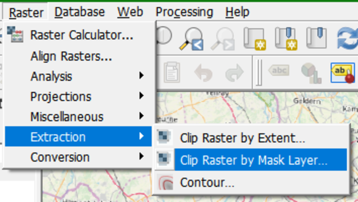
6. In the Clip Raster by Mask Layer dialogue, choose dem_reprojected for the Input layer. For Mask Layer, choose boundingbox. Keep the defaults for the other options. Choose dem_subset for the Clipped (mask) output and click Run. Click Close when done.
Often you'll not have a bounding box shapefile. In that case you can choose Raster | Extraction | Clip Raster by Extent. Then you can drag a box in the Map Canvas and use that for clipping. While using that, make sure your on-the-fly reprojection is similar to the layer that you want to clip, because the Map Canvas coordinates are used by the algorithm.
7. Now you can remove dem_reprojected from the layers list as we have done before for other layers that are no longer needed.
6.1. Styling the DEM
The default legends produced by Desktop GIS software are often not
intuitive, because the software does not know (1) what information is
presented, and (2) the raster data type (e.g. Boolean, discrete or
continuous data). To help interpret the results it is good practice to
style your layers intuitively.
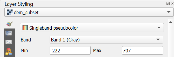
The DEM is a continuous raster. Continuous rasters represent gradients and can therefore contain real numbers (or floating point). Continuous rasters are styled in QGIS using ramps in the Singleband pseudocolor dialogue.
1. Select the dem_subset layer and click ![]() to open the Layer Styling panel (or press
to open the Layer Styling panel (or press F7).
2. In the Layer Styling panel choose Singleband pseudocolor
from the drop-down list.
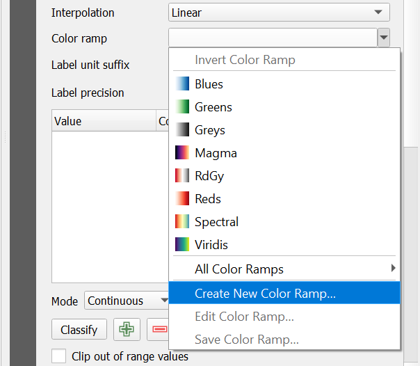
3. Click the arrow at Color ramp and choose Create New Color Ramp from the dropdown menu.
4. In the popup Color ramp type dialogue choose Catalog: cpt-city from the drop-down list.
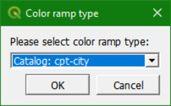
The cpt-city catalogue has a lot of useful preset color ramps.
5. Choose Topography | Elevation. Note that cd-a and sd-a are also nice choices.
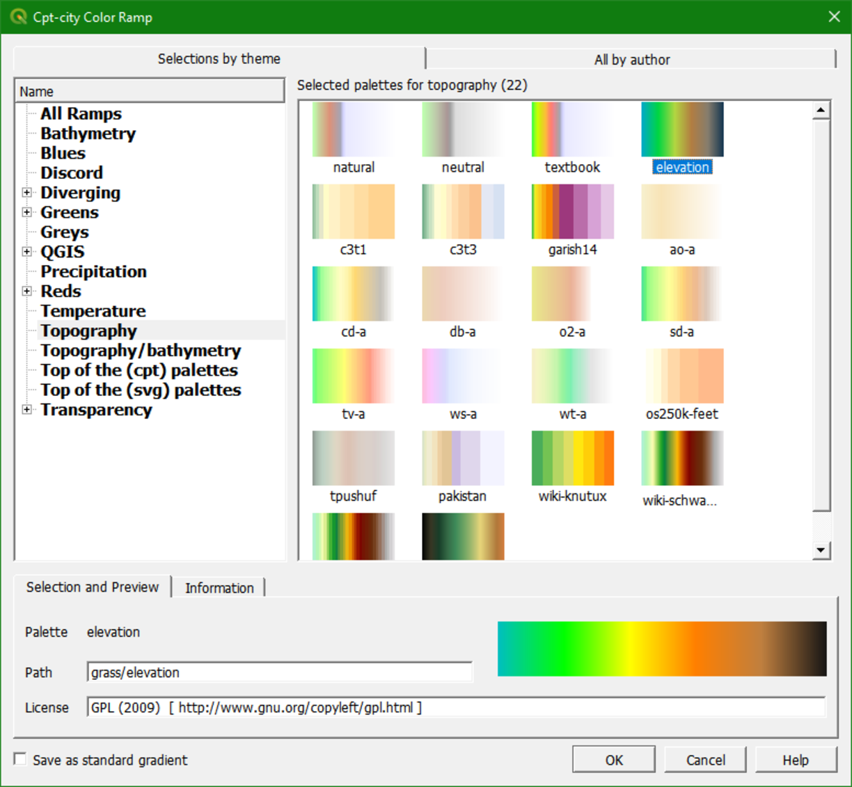
6. Click OK.
7. Now click Classify to apply the color ramp.
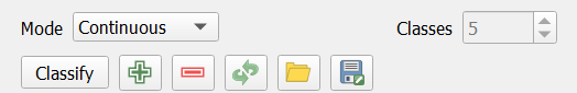
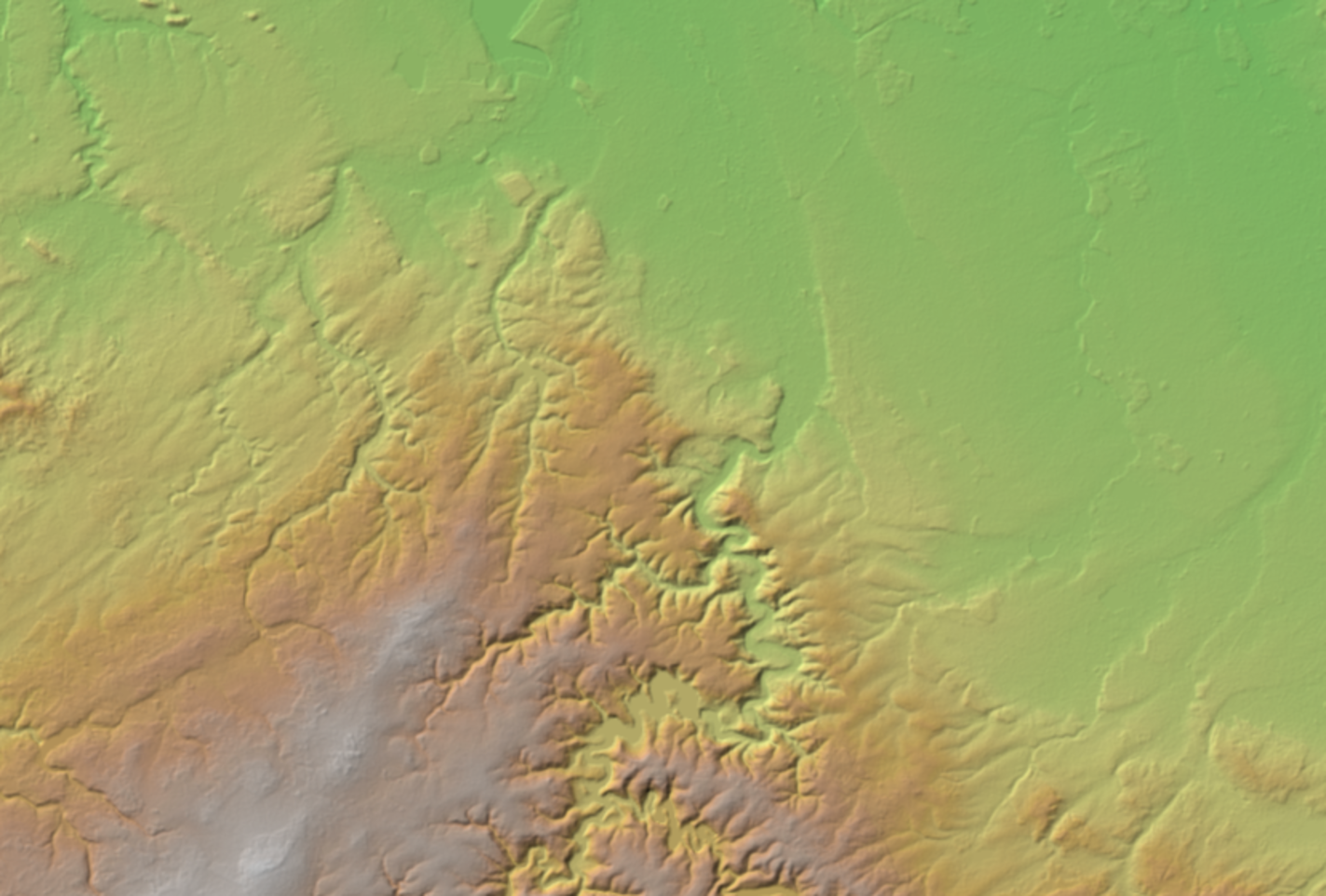
This gives us more intuitive colors in the DEM where we can clearly distinguish higher and lower areas. Now we will further improve the visualisation.
8. Right-click on the dem_subset layer in the Layers panel and select Duplicate Layer.
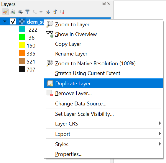
This creates a copy of the dem_subset layer called dem_subset copy.
9. Uncheck the dem_subset layer, check the dem_subset copy layer and rename it to hillshade.
10. In the Layer Styling panel, which should still be open, make sure that the hillshade layer is now selected. In the drop-down list change Singleband pseudocolor to Hillshade.
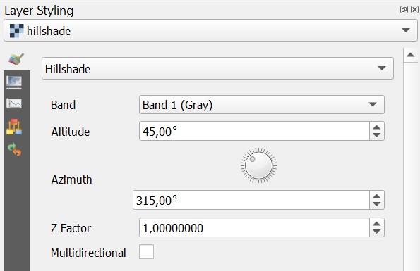
Now the hillshade layer is visualised with a shading.
Which direction is the illumination coming from? Is this possible in reality?
Hillshade gives the best results with an artificial illumination in the northwest, which in reality can not exist in the Northern Hemisphere. If you move the dial in the Layer Styling panel to the southwest, you will see an inverted relief. Also note that there is a Resampling section. The default resampling method for both Zoomed in and Zoomed out is Nearest Neighbor. This method is fine for categorical data however, elevation is considered continuous data. You should therefore choose a Zoomed in resampling method of Bilinear and a Zoomed out resampling method of Cubic.
Next, we're going to blend the DEM with the hillshade layer.
9. Switch on the dem_subset layer by checking the box.
10. In the Layer Styling panel make sure the dem_subset layer is selected. In the Layer Rendering block of the panel, change the Blending mode to Multiply.
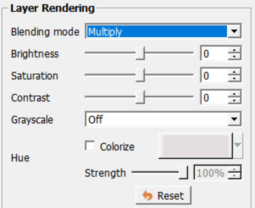
As you can see, blending gives a much nicer effect than transparency. With transparency the colors will fade. Now we can clearly see the elevation differences: the gradient from south to north and the valleys where we expect the streams.
Blending modes allow for more elegant rendering between GIS layers. They can be much more powerful than simply adjusting layer Opacity. Blending modes allow for effects where the full intensity of an underlying layer is still visible through the layer above. There are 13 blending modes available. See here for more info.
7. Fill Sinks and Calculate Flow Direction
Raw, unprocessed DEMs have artifacts such as depressions. Artifacts are a result of the DEM acquisition process and must be removed before a DEM can be used for hydrological analysis, like catchment and stream delineation or hydrological modelling. There are several algorithms for filling sinks. Here we'll use the lddcreate tool of PCRaster. This tool fills the sinks and creates a flow direction map (also called local drain direction map) that can be used in the next steps.
7.1. Install the PCRaster Tools plugin
PCRaster is a powerful package of software for map algebra and environmental dynamic modelling. The main applications of PCRaster are found in environmental modelling: geography, hydrology, ecology to name a few. An extensive set of raster operations is available: several point operations (analytical and arithmetical functions, Boolean operators, operators for relations, comparison, rounding, field generation etc.), neighbourhood operations for calculations in moving windows (highpass filtering, edge filtering, moving averages, etc.), area operations for calculations within specified areas (for instance soil groups), operations for the calculation of cost paths. In the PCRaster package a rich suite of geomorphological and hydrological functions is available. These include functions for visibility analysis, catchment analysis and routing of transport (drainage) of material in a catchment using interactively generated local drain direction maps and transport (routing) operations. These operations are made available in the QGIS Processing Toolbox through the PCRaster Toolsplugin.Before you can install the PCRaster Tools plugin you need to install PCRaster.
On Windows you can install PCRaster with the OSGeo4W installer. This video shows the procedure:
- Run the OSGeo4W setup which comes with your QGIS version
- Choose Advanced Install, click Next
- Choose Install from Internet, click Next
- Select the root install directory or keep the defaults, click Next
- Select local package directory or keep the defaults, click Next
- Select your internet connection, click Next
- Choose one of the download sites, click Next
- In the Select Packages window search for
pcraster - Click the arrows icon to change from skip to a PCRaster version to install.

pcraster and install the PCRaster Tools plugin.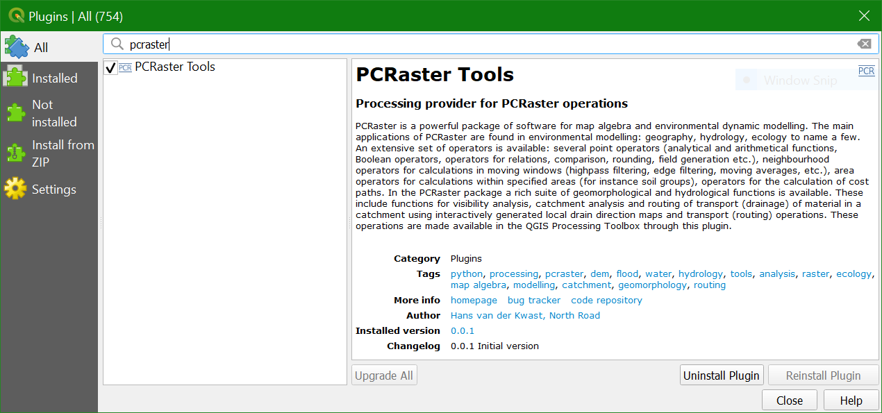
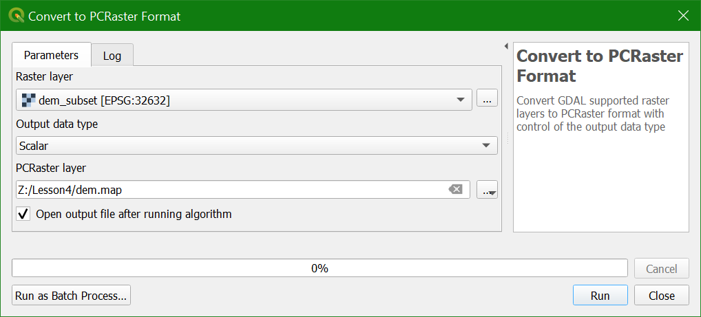
7.2. Convert GeoTIFF to PCRaster Format
In order to use the PCRaster tools we need to convert raster to the PCRaster map format, which is a GDAL supported format. This is needed, because PCRaster is strict with data types.
PCRaster distinguishes the following raster data types:
- Boolean: cells are 0 (False) or 1 (True)
- Nominal: cells have positive integer values representing classes (discreet raster) without a specific order, for example land-use classes
- Ordinal: cells have positive integer values representing classes (discreet raster) with a specific order, for example stream order.
- Scalar: cells have real values (decimal, positive, negative). This is used for continuous rasters.
- Directional: for rasters with a compass direction (e.g. aspect).
- LDD: local drain direction, a specific data type for flow direction rasters
7.3. Calculate the Flow Direction
The next step is to fill the sinks (artificial depressions in the DEM) and calculate the flow direction raster. PCRaster does both in one step with the lddcreate tool. Check the documentation for the details.
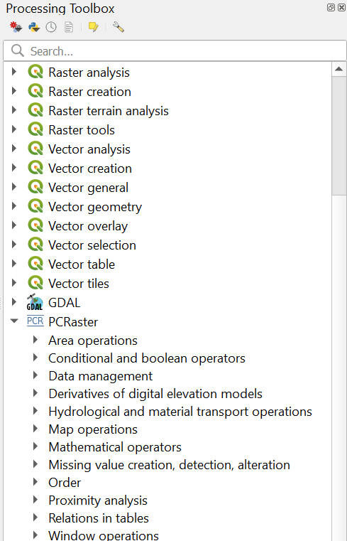
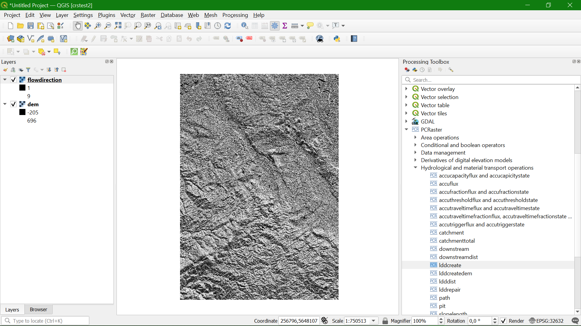
1. In the Processing Toolbox go to Hydrological and material transport operations | lddcreate
2. In the Lddcreate dialogue choose dem as DEM layer. Keep all other defaults so it will fill the sinks completely. Save the results to flowdirection.map.
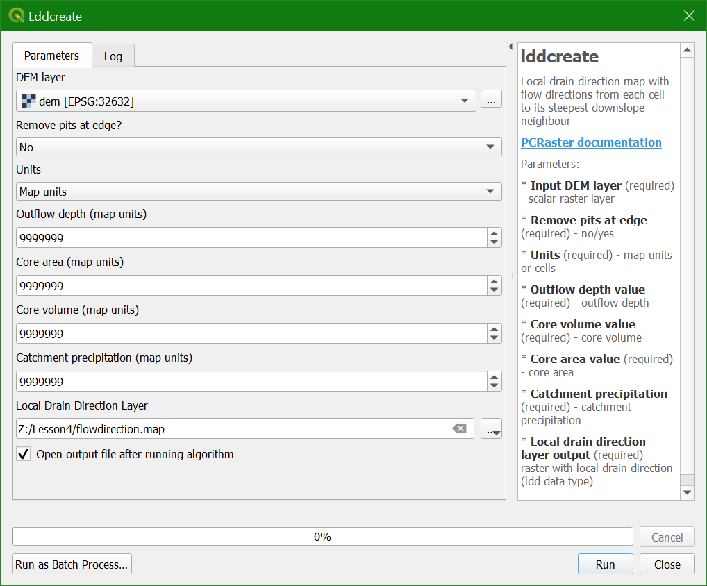
3. Click Run. This can take a few minutes before the result appears in the map canvas. Click Close to close the dialogue.
In the next step we'll style the flow direction map.
A
flow direction layer indicates the direction of flow for each pixel.
Direction can be expressed as compass direction, however we can not
store text in a raster. Compass direction can also be expressed by
degrees on a circle where north is 0 degrees, east is 90 degrees, etc.
To store 360 degrees we would need more than 8 bits (0-255), which would
increase the file size. In addition the D8 method uses discrete
directions to the surrounding pixels. Therefore GIS software recodes the
8 directions. Each software, however, does it in their own way. The PCRaster lddcreate algorithm used in the QGIS Processing Toolbox uses the values of the numeric keypad for the directions.
7.4. Styling the Flow Direction Layer
Next you will work on styling the flow direction raster. This will help you check the results and ensure they match what you were expecting. You will employ a circular color ramp to intuitively show southern oriented flows with warm colors and northern facing flows with cool colors.
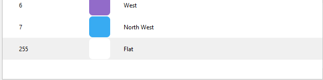
Because the flow directions in the PCRaster LDD format are in a complicated order to style (numbers on the numeric pad), we'll first reclassify the flow direction values using the values used by SAGA (0 = North, 1 = North East, ..., 7 = North West, 255 = Flat).
1. In the Processing Toolbox go to Raster Analysis | Reclassify by table
2. In the Reclassify by Table dialogue choose flowdirection as Raster layer and click  at Reclassification table to create the lookup table.
3. Fill in the table as the screenshot below and click OK to return to the main dialogue.
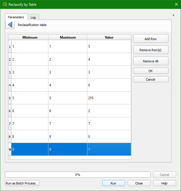
4. Change the Range boundaries so they include the min and max values, choose Byte for Output data type (1 byte = 8 bits = 256, which is enough to store the flow direction values) and save the Reclassified raster to flowdir.tif.
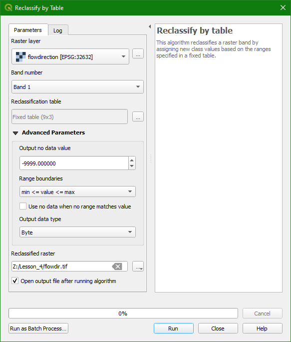
5. Click Run to perform the reclassification. Click Close to close the dialogue.
6. Using the Layer Styling panel set the target layer to flowdir.
7. Set the renderer to Paletted/Unique values and click Classify.
8. Since the value of 255 represents flat surfaces, select that value and click the Minus  button to remove it from the classification.
9. Choose the Spectral color ramp as a beginning point. Right-click on the color ramp and choose Edit Color Ramp.
10. The Select color ramp window will open. Here you can edit the color stops for the ramp. The idea is that the far left and right sides will represent northern flows and you will set both of those stops to the same blue color. You will then set the center stop to a bright yellow for southern flows. The stop in the middle on the right will be western flows and the stop in the middle to the left will be eastern flows.
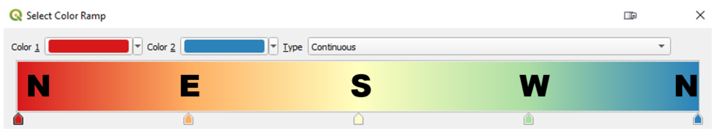
11. Click the drop-down menu for Color 1 and choose Pick color from the context menu. With the eye dropper cursor click on the Color 2.
12. Click the center stop that will represent southern flows and assign it a bright yellow by entering these RGB values: 255 | 255 | 0.
13. For the eastern stop assign the color green by entering these RGB values: 0 | 255 | 0.
14. For the western stop use a magenta color, RGB: 214 | 60 | 170.
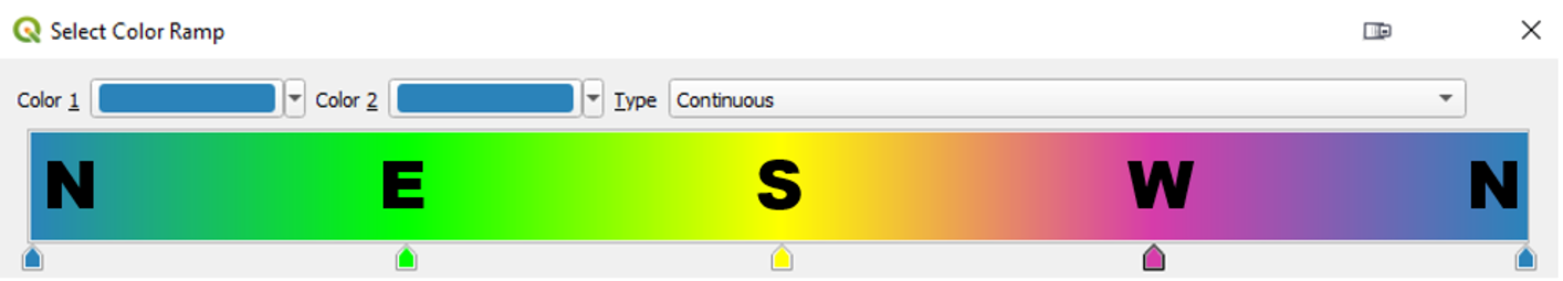
Note that the last stop in fact will represent NW. Therefore you could improve the ramp by giving the last stop a colour between magenta of west and blue of North.
15. Click OK to accept the new color ramp.
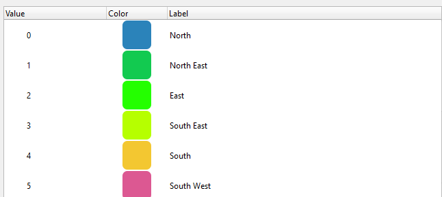
16. Click the Plus ![]() button to add a new value to the classification for the Value type 255. This represents the flat areas you initially removed before creating the circular color ramp. Click the color patch and choose white.
button to add a new value to the classification for the Value type 255. This represents the flat areas you initially removed before creating the circular color ramp. Click the color patch and choose white.
17. Edit the labels in such a way the reflect the compass directions in a human readable way, instead of the pixel values.
18. To review the flowdir data you will now give it a Blending mode of Multiply and turn on the hillshade layer. This will allow you to see the detail of the hillshade through the flowdir layer. At this point just have the channels, flowdir, and hillshade layers turned on. Zoom in to some of the more mountainous terrain in the south of the study area where there are also channels present. Inspect the data.
You should see southern facing slopes being represented by warmer colors and northern by cooler colors, eastern flows will be greener and western flows more purple.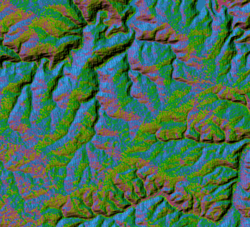
8. Delineate Streams
Now we have the flow direction we can proceed with delineating the streams.
First we'll calculate the Strahler Orders, then we'll calibrate the Strahler threshold to determine the streams.
8.1. Calculate Strahler Orders
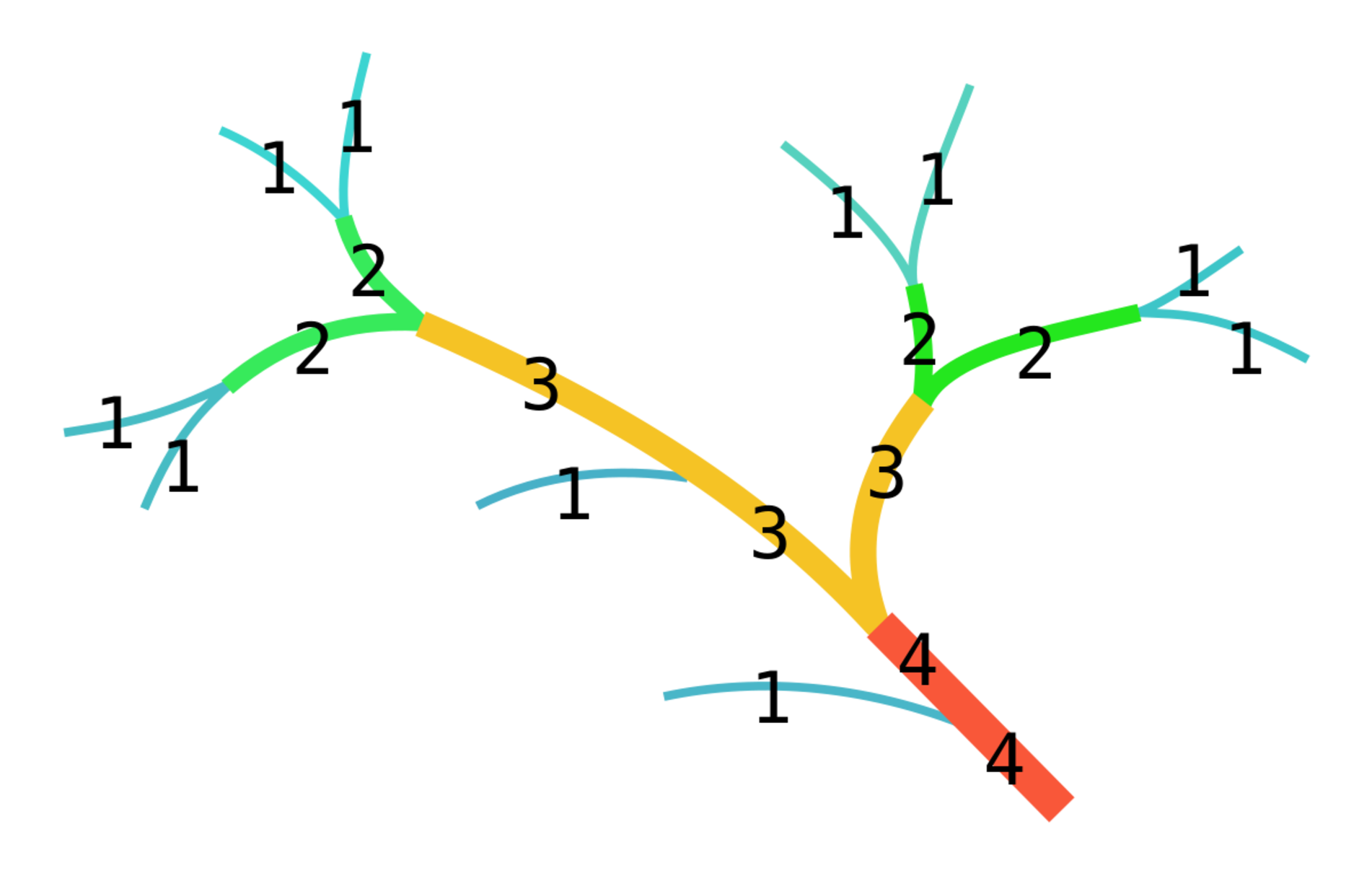
Before we can derive the streams from the DEM, we need to determine what we consider streams. For this purpose we use the Strahler order. The higher the order, the bigger the stream.
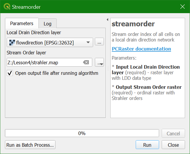
1. Search for streamorder in the Processing Toolbox and select PCRaster | Hydrological and transport operations | streamorder.
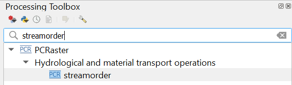
2. In the Streamorder dialogue, select flowdirection for the Local Drain Direction layer, use strahler.map as the Stream Order output filename, and click Run. Click Close when the algorithm is done.
To make more sense of the strahler layer we are going to style it.
Is the Strahler order layer a Boolean, discrete, or continuous raster?
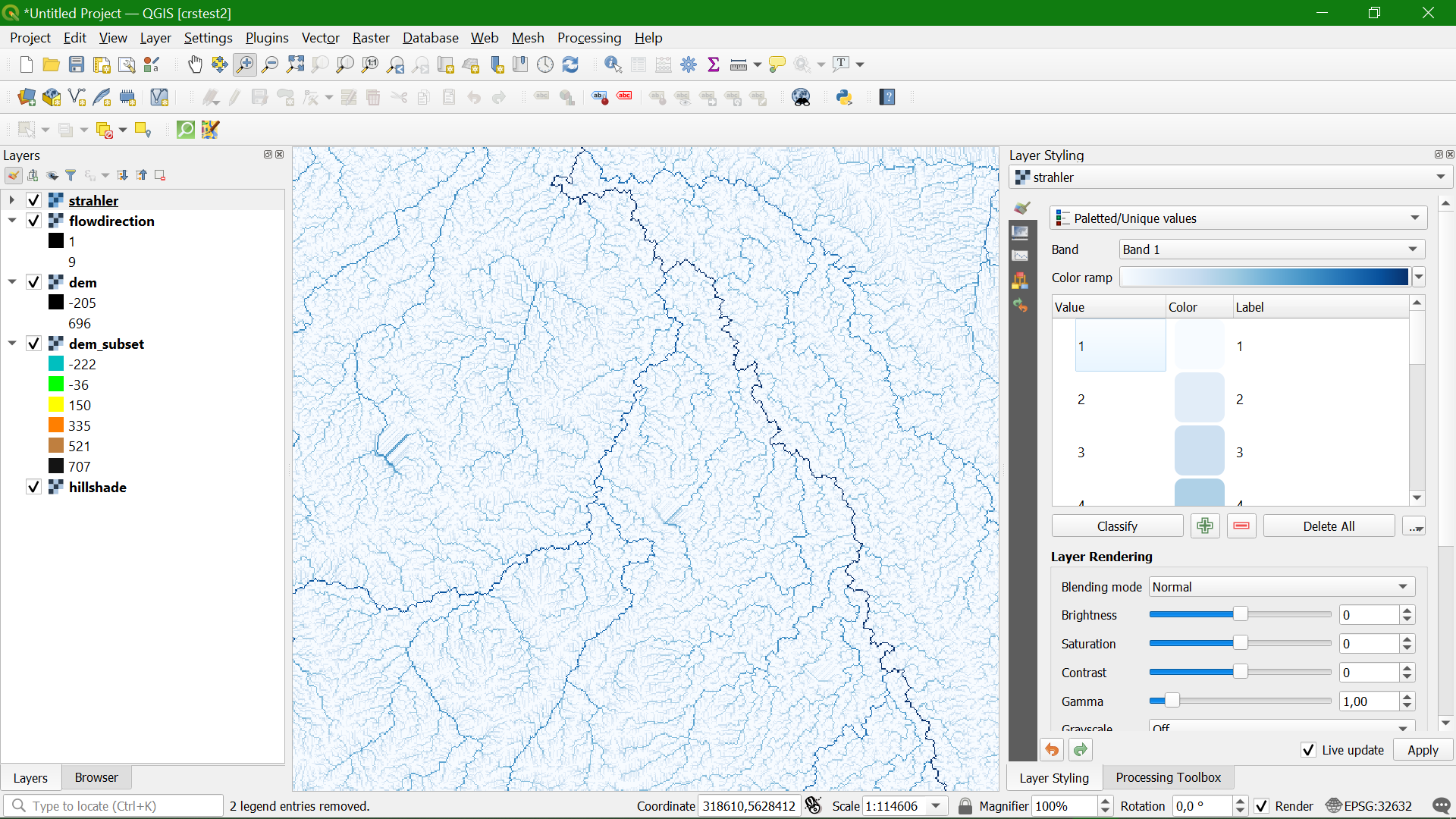
The Strahler order layer is a discrete raster, but the order of the classes is important. Therefore for PCRaster it has the ordinal data type. For discrete rasters in QGIS we use the Paletted/Unique values styling. The higher the Strahler order, the bigger the stream. So we will use a color ramp from white to blue.
3. Open the Layer Styling panel if you closed it before and make sure that the strahler layer is selected.
4. Choose Paletted/Unique values from the drop-down menu.
5. Click Classify.
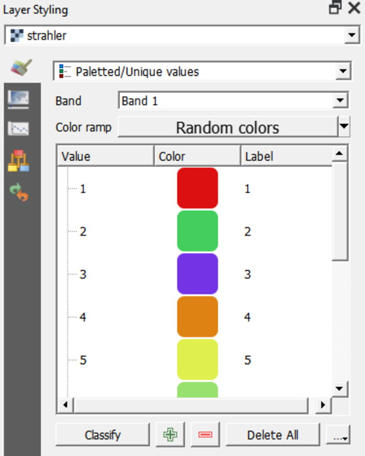
To each unique value in the raster a unique random color has been assigned.
6. Right-click on Random colors and choose Blues.
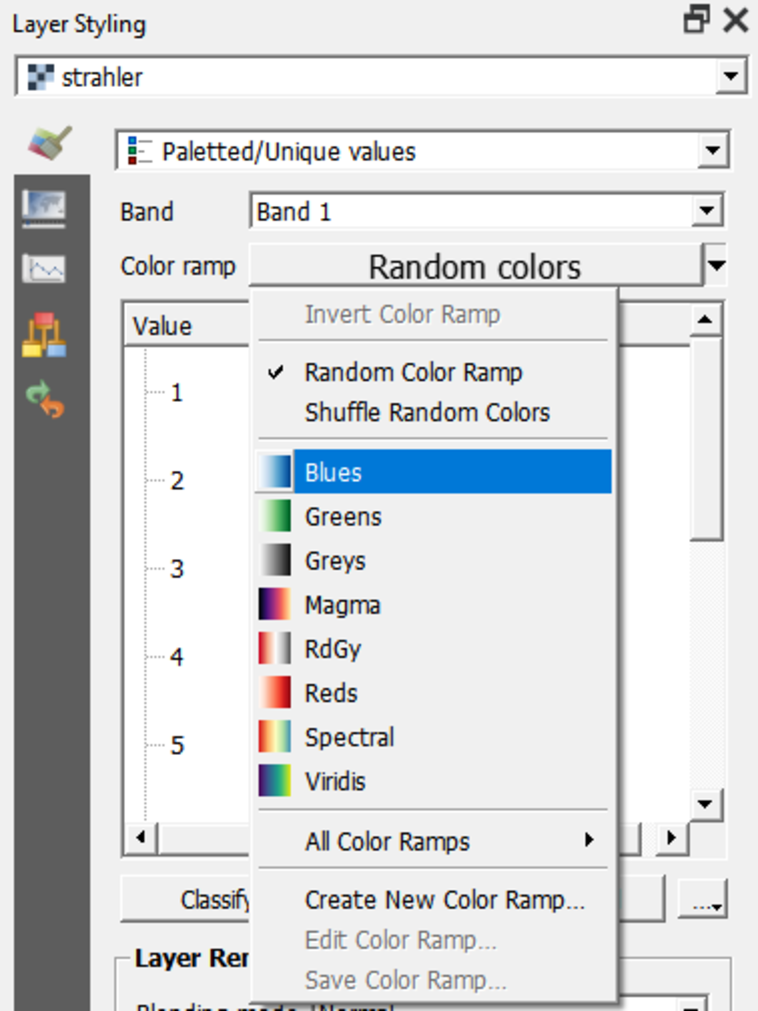
The strahler layer now shows in an intuitive way that the higher orders will be larger streams than the lower orders.
8.2. Calibrate Strahler Threshold to Determine Streams
The next step is to apply a calibration procedure to determine which Strahler orders we consider to be streams. We will create Boolean layers for Strahler orders larger than or equal to a threshold value. Each Boolean layer will be compared with a reference layer. Here we will compare the Strahler orders with the rivers on OpenStreetMap. For areas where there is a lack of data in OpenStreetMap, you could use the Google Satellite. Both OpenStreetMap and Google Satellite layers can be found in the QuickMapServices plugin.2. Fill in the dialogue as in the figure below. Call the output file
strahler5.tif and click OK to run the calculation.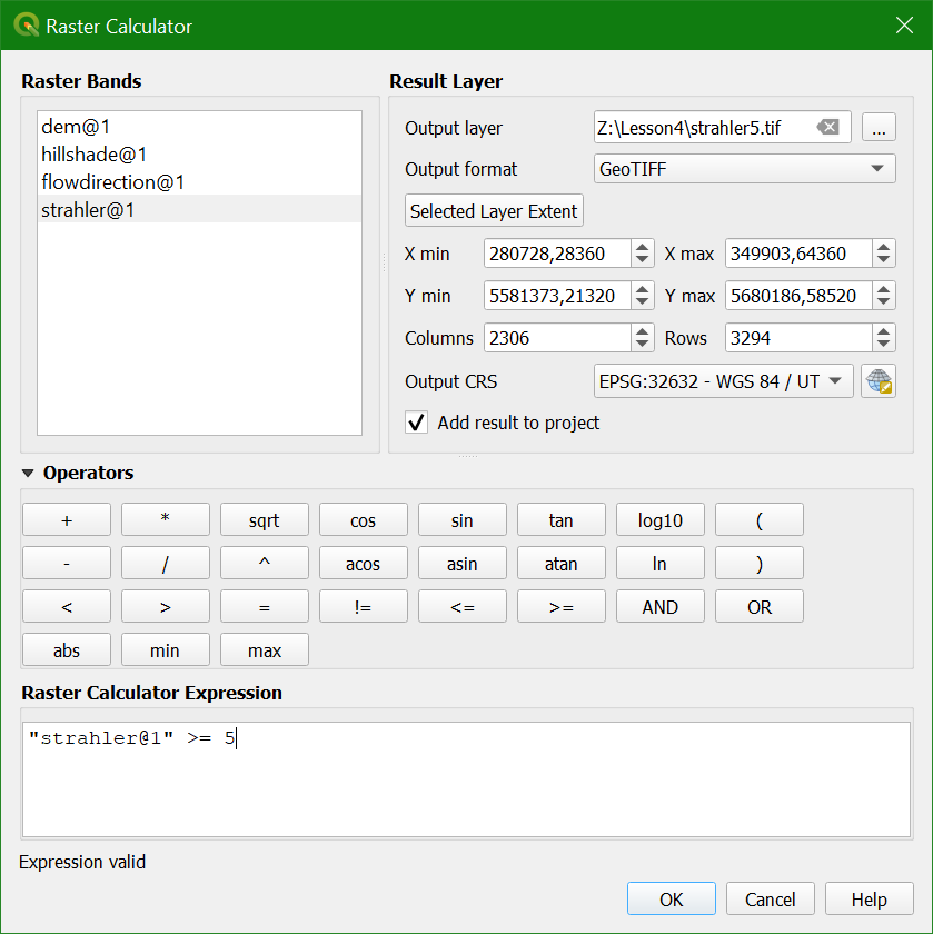
It is also good practice to style the strahler5.
3. Go to the Layer Styling panel and make sure that strahler5 is selected.
4. Choose Paletted/Unique values from the drop-down menu.
This layer is Boolean and therefore it has only pixels with values 0 and 1. For our calibration it is important to make the zeros transparent and the ones blue so we can compare the raster with the streams on OpenStreetMap.
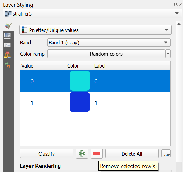
In the Map Canvas we can see now all streams larger than or equal to Strahler order 5 and we can compare them with the rivers on the OpenStreetMap.
8. Repeat the steps in this subsection for different Strahler order threshold values and determine the one that corresponds best with the rivers on OpenStreetMap. Remove the other Boolean layers.
Tip: You can copy the styles of the layers: right-click on a layer, choose Styles | Copy Style and then right-click on the target layer and choose Styles | Paste Style.
8.3. Calculate Channel Network
The next step is to calculate the channel network, based on the Strahler threshold determined in the previous step.
First we're going to create a layer with the Strahler orders for the rivers by selecting the cells with order equal to or higher than the threshold determined in the previous step. Here we'll use order 8 as threshold.
With the spatial tool you can make rasters with for all cells the input nonspatial value and the chosen data type.
1. Create an ordinal layer with value of the threshold, i.e. 8. In the Processing Toolbox go to PCRaster | Data management | spatial
2. In the Spatial dialogue type 8 for Input nonspatial. Choose Ordinal for Output data type and strahler as the Mask layer. Call the Output raster layer ordinal8.map.
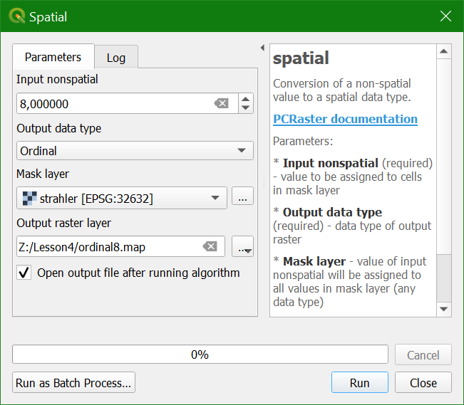
3. Click Run and Close the dialogue after completion.
Now we're going to create a boolean layer with 1 (True) for all strahler cells that are >= 8:
4. In the Processing Toolbox go to PCRaster | Conditional and boolean operators | comparison operators.
5. In the Comparison Operators dialogue choose strahler as Input raster, >= as Comparison operator and ordinal8 as the second Input raster.
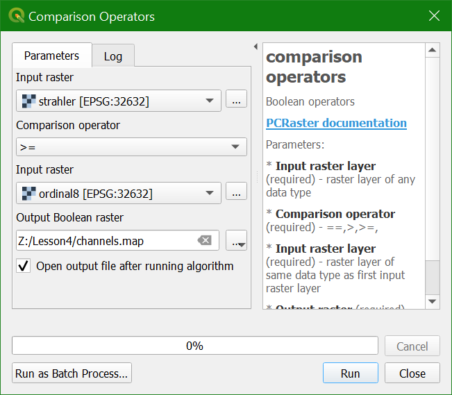
6. Click Run and Close the dialogue after processing.
Now we have a boolean layer with the channels that we can use now to assign the river strahler orders.
7. In the Processong Toolbox go to PCRaster | Conditional and boolean operators | ifthen
8. In the If Then dialogue choose channels as the Input Boolean Condition Raster and strahler as the Input True Raster. Call the Output raster channelsstrahler.map.
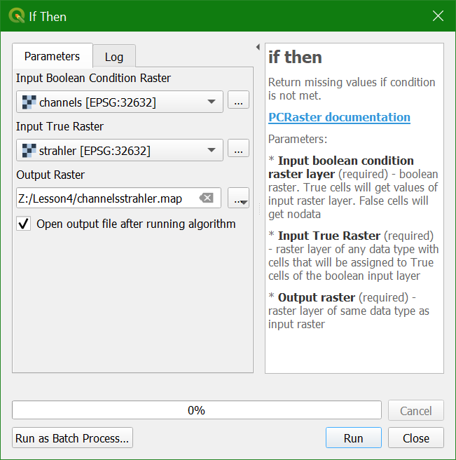
9. Click Run and Close the dialogue after processing.
Now we have a raster with the Strahler orders for the channels. This can be visualised better as a vector, whick will be explained in the next section.
8.4. Convert Raster to Vector Lines
For better visualisation of the channel network, we need to convert the channelsstrahler layer to a line vector.
We'll use the GRASS tools from the Processing Toolbox for this.
First we need to thin the raster lines, so they are only 1 pixel wide.
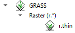
1. From the Processing Toolbox choose GRASS | Raser (r.*) | r.thin
2. In the r.thin dialogue choose channelsstrahler as Input raster layer to thin. Keep the defaults and save the Thinned raster as channelsthin.tif.
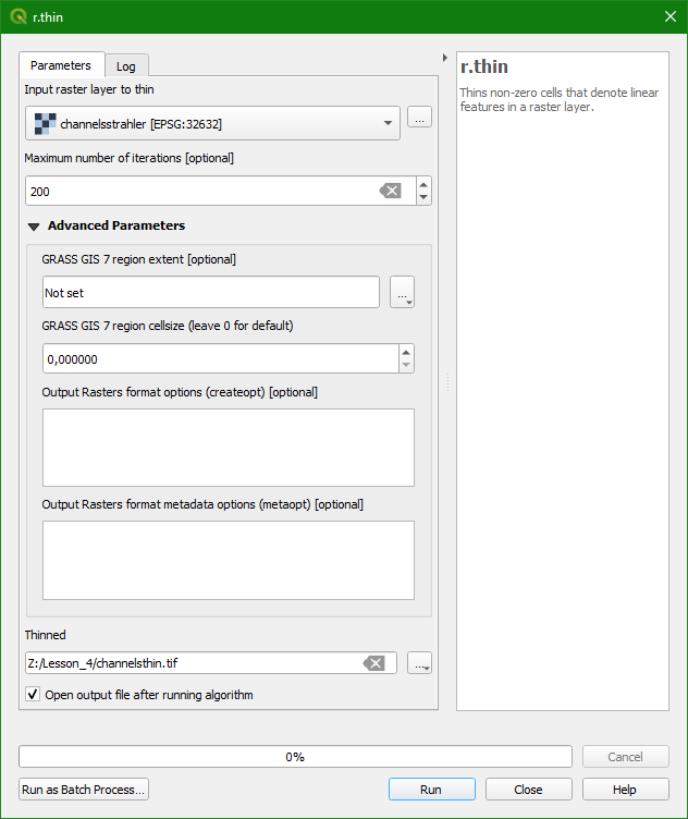
3. Click Run to perform the thinning and click Close when the processing is completed.
4. Compare the result with the channelsstrahler layer to understand what r.thin does.
Now we can convert the channelsthin layer to a line vector.
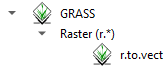
5. In the Processing Toolbox go to GRASS | Raster (r.*) | r.to.vect
6. In the r.to.vect dialogue
- choose channelsthin as Input raster layer
- choose line from the drop down menu as Feature type
- check the box to Use raster values as categories instead of a unique sequence
- under Advanced Parameters change the v.out.ogr output type to line
- name the Vectorized output channels.shp
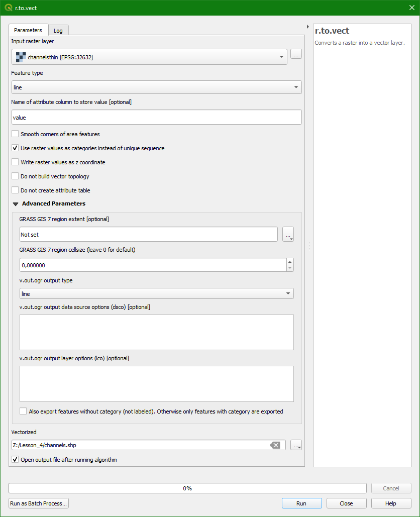
7. Keep the rest as default. Click Run to perform the conversion. Click Close when the processing is done.
The result has some geometrical errors that can be fixed using v.clean from the Processing Toolbox or the Topology Checker plugin. This is not covered in this tutorial.
In the next section we'll style the channels layer.
8.5. Styling the channels
Next you will style the channels to get a better understanding of the results.
1. Open the attribute table of the channels layer.2. Click the Field calculator button 
3. In the Field Calculator dialogue create a new field ORDER with Output field type Whole number (integer) and Output field length 1. Under Expression write the code as given below:
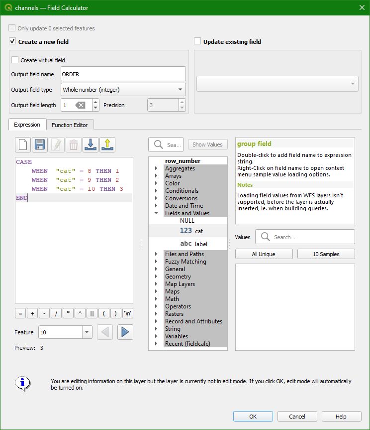
4. Click OK.
5. Toggle off editing by clicking  and save the edits. Close the attribute table.
6. Open the Layer Styling panel and set the target layer to channels.
7. Choose the Graduated renderer with the following settings:
- Set the Value to ORDER and the Precision to 0 since Strahler Order values are integers.
- Set the Method to Size.
- Set the Size from values from
0.3to1.0mm. - Set the Mode to Equal Interval with the same number of Strahler Order classes that exist in your data. Review the attribute table if need be. In this example it is set to 3 classes. Click Classify.
- Set the Legend values to integer Strahler order values. Note that the first range always includes both the minimum and maximum value. The other ranges exclude the minimum value and include the maximum value.
8. Click the Change button and set the Color to an RGB value of 15 | 66 | 220.
9. Click the Go back ![]() button to return to the main symbology panel.
button to return to the main symbology panel.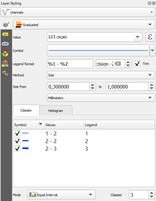
You might have noticed the the lines are not very smooth as river lines should be. We'll make them smoother to make them look more realistic.
10. In the Processing Toolbox click the Edit features In-Place button  . This will select tools that can be applied to vector layers without saving a copy.
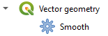
11. Look for the Vector geometry | Smooth tool.
12. In the Smooth dialogue change the Iterations to 5 (the higher the number, the smoother the line). Keep the other values as default and click Modify All Features.
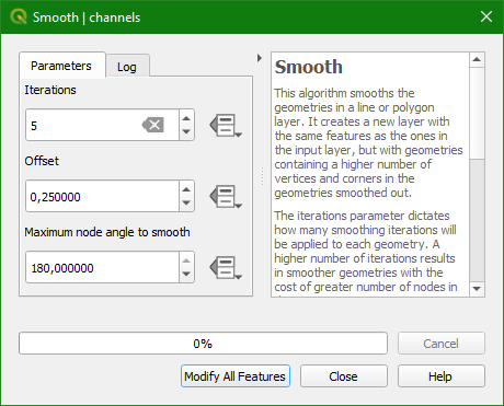
13 Click Close.
14. Toggle off editing mode and save the edits.
15. Click  to deselect all features.
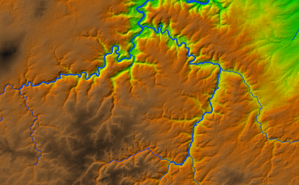
Your map should now resemble the figure below, showing the streams identified as having higher Strahler Orders are the main channels and the smaller ordered streams
are tributaries.
9. Define Outflow Point
A catchment is an extent or an area of land where surface water from rain, melting snow, or ice converges to a single point at a lower elevation, usually the exit of the basin, where the waters join another water body, such as a river, lake, reservoir, estuary, wetland, sea, or ocean. In order to delineate a catchment we need to have:
- the coordinates of our outlet in the same coordinate system as the map we are using
- the channel network that matches the flow directions as calculated from a hydrologically correct DEM
The outflow point of the Rur catchment is in Roermond, where the Rur enters the Meuse river (Maas in Dutch). The channel network that has been derived in the previous step is in the channels layer.
1. Make sure you have the channelsstrahler layer on top of the OSM Standard layer from the QuickMapServices plugin.
2. Look for the location where the Rur river flows into the Meuse. Note that on the OpenStreetMap the Dutch names are used, because it lies in the Netherlands. Rur is spelled as Roer and Meuse is spelled as Maas.
Note that the delineated channels are not corresponding well with the channels on OpenStreetMap. This can be for the following reasons: (1) Incorrect automatic delineation of streams, which can be caused by errors in the DEM or areas that are too flat, (2) Distortion due to (on-the-fly) reprojection and (3) Human influence on the natural course of the channels. The catchment delineation, however, only works when the outlet is defined on a delineated channel, because that corresponds with the filled DEM.
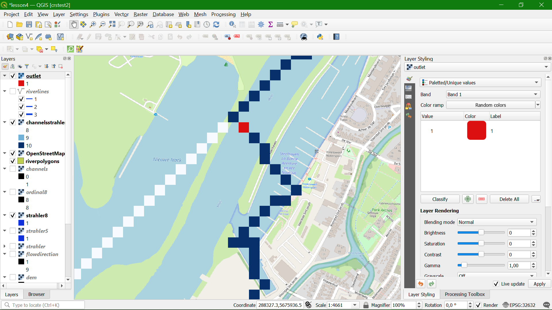
3. Choose a point on the delineated channel that is close to the real outlet of the Rur in the Meuse (step 2).
4. Click right on the pixel and copy the coordinate.
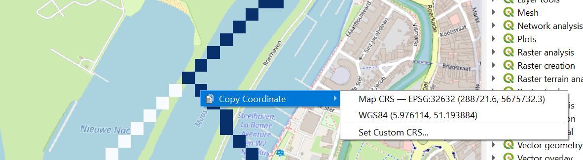
5. Paste the coordinates in a text editor (e.g. Notepad) and add a comma and a 1:

We've added the ID 1 to the coordinate. You can add more outlets to the file with unique ID's if you want to delineate (sub)catchments for multiple outlets.
6. Save the file as outlet.txt.
7. In the Processing Toolbox go to PCRaster | Data management | Column file to PCRaster Map.
8. In the Column File to PCRaster Map dialogue browse to the text file with the outlet, choose flowdirection as the Raster mask layer, choose Nominal as the Output data type and save the file as outlet.map.
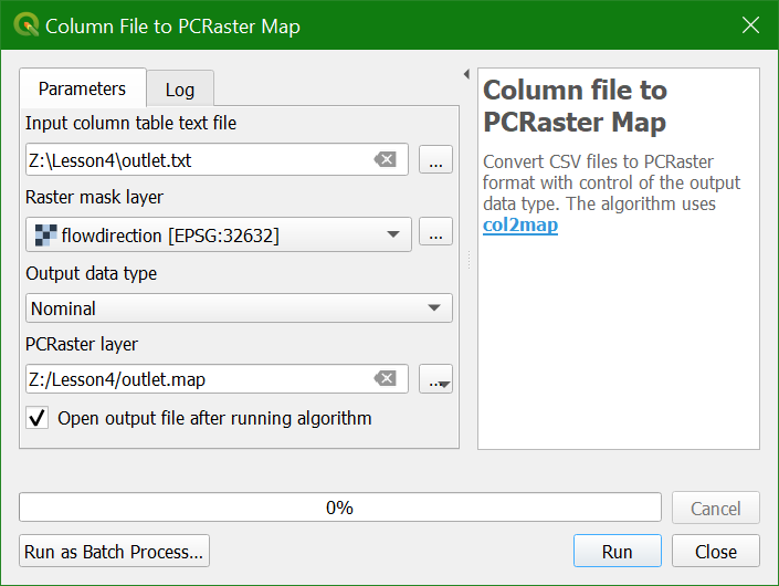
9. Click Run and Close after processing.
Now the outlet point has been added to the map canvas.
10. style the point with a clear colour using the paletted/unique values renderer.
In the next section we'll delineate the catchment of this outlet.
10. Delineate the Catchment
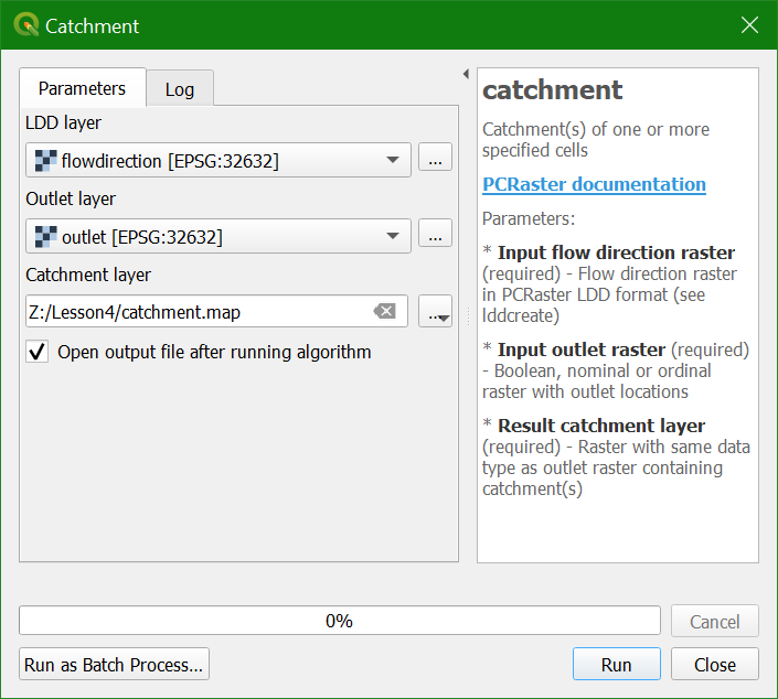
3. Click Run and Close the dialogue after processing.
The result should look like the screenshot in the figure below if you zoom to the extent of the layer. The result is a boolean layer with cell value 1 for the catchment and 0 for outside the catchment.
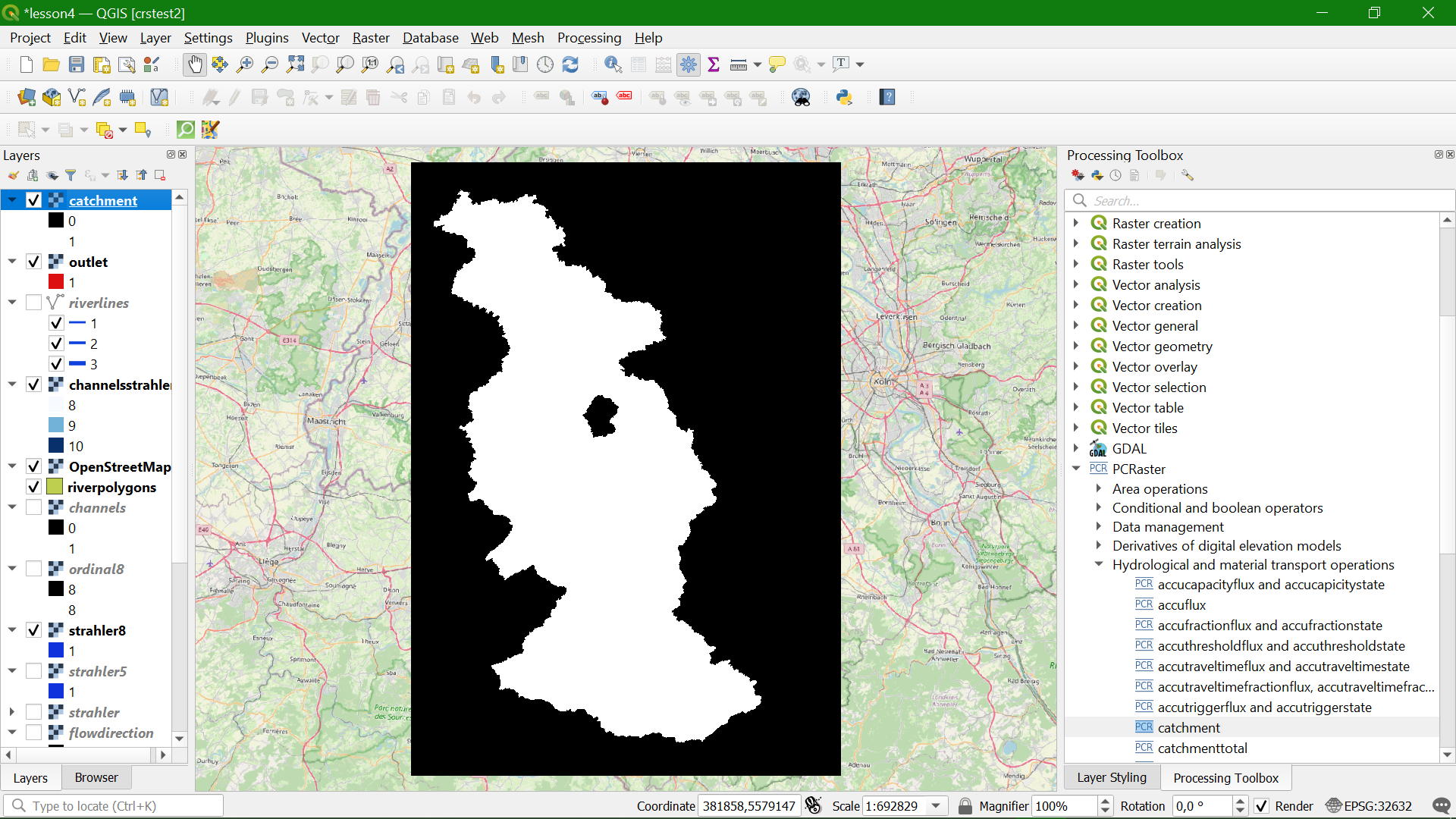
In order to overlay the catchment boundary with other data, it is better to convert it from raster to vector (polygon).
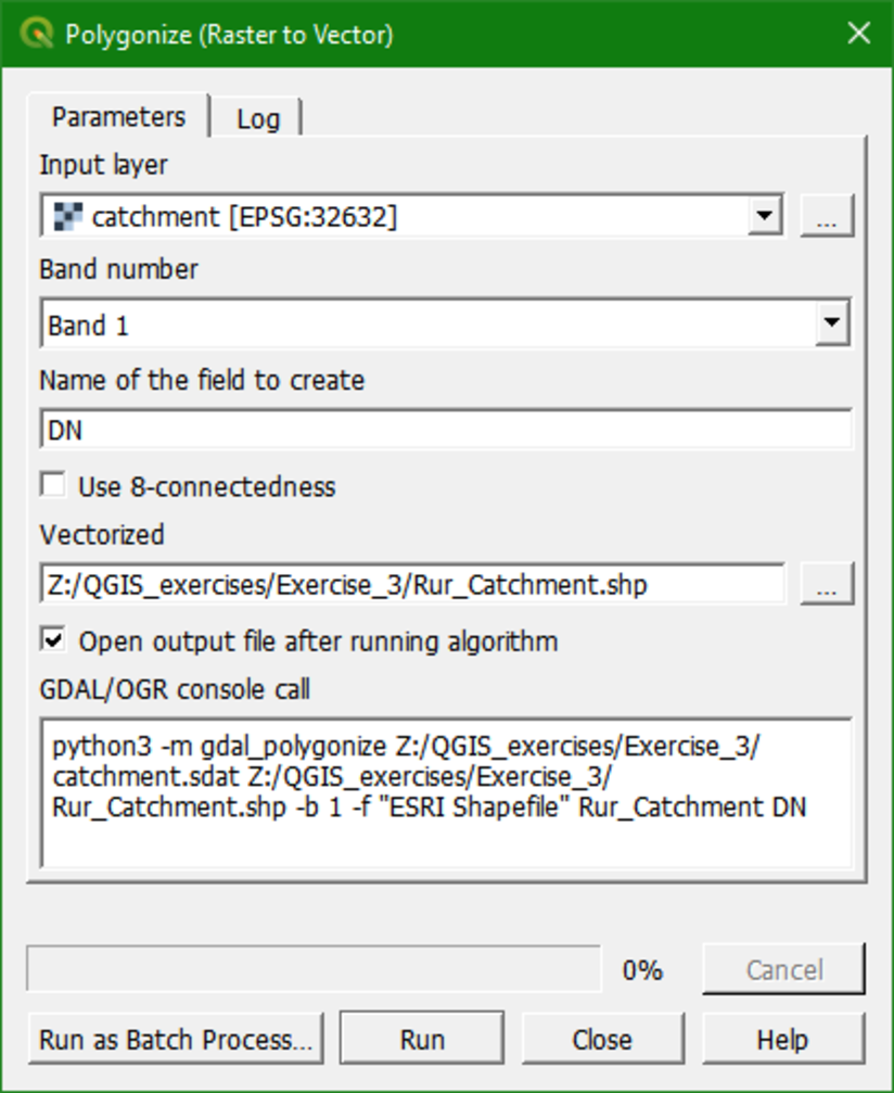
4. To convert the raster layer to vector, go to the main menu and choose Raster | Conversion | Polygonize (Raster to vector).
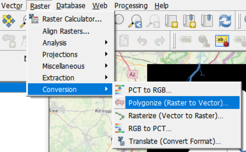
5. Make sure you choose the right input and call the output Rur_catchment.shp. Click Run. Click Close to get back to the main screen.
6. Look at the result. Also check the attribute table (right-click on layer name and choose Open attribute table).
7. In the attribute table, toggle to editing mode using the ![]() button, then select the record that you want to remove by clicking on the row. The selection will be highlighted in yellow on the map. Click the
button, then select the record that you want to remove by clicking on the row. The selection will be highlighted in yellow on the map. Click the ![]() button to delete the selected feature, toggle off editing by clicking
button to delete the selected feature, toggle off editing by clicking ![]() again, and save the changes.
again, and save the changes.
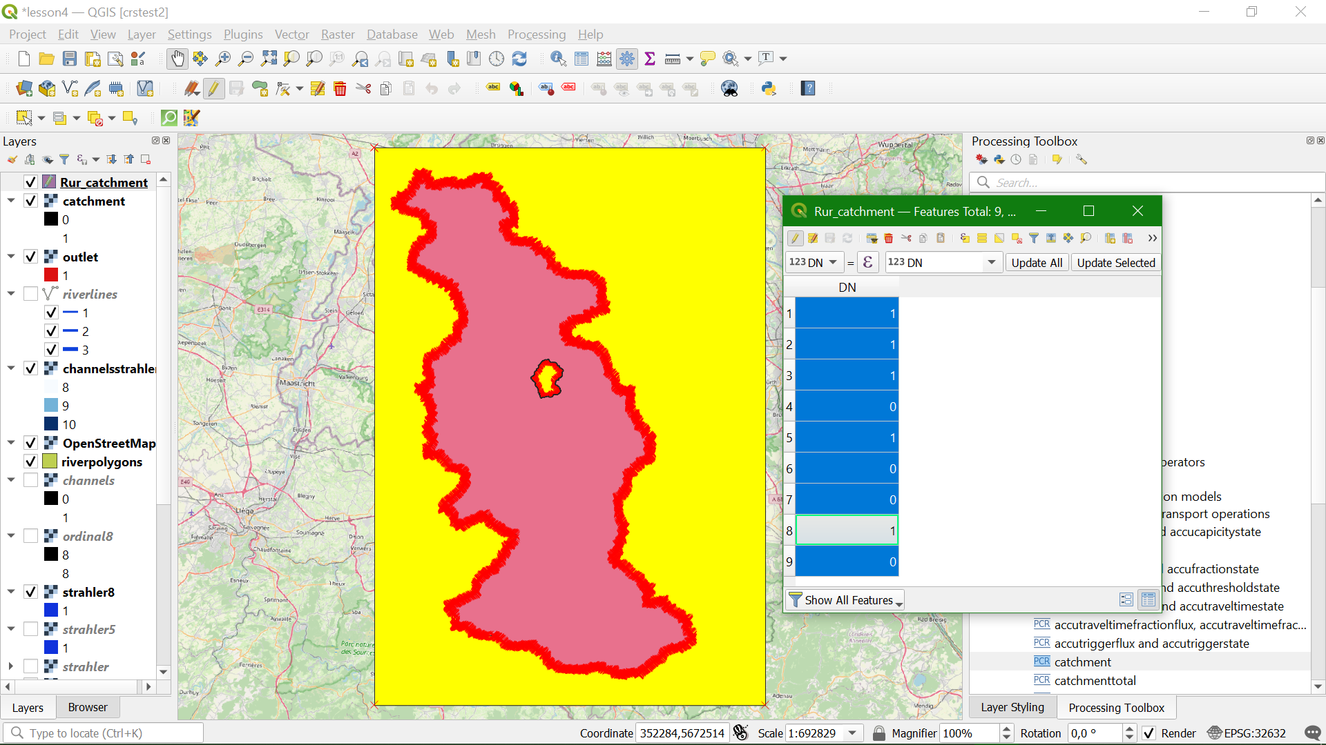
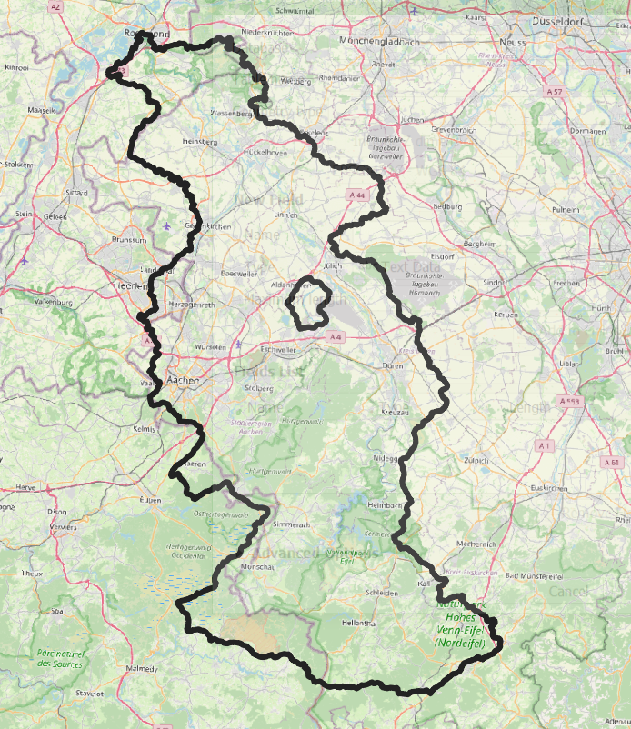
Now the catchment map should look like this after styling.
11. Clipping layers to the catchment boundary
Now that we have a boundary polygon, we can clip the channels and DEM to this boundary.
Let's start with clipping the channels.
1. In the main menu, go to Vector | Geoprocessing Tools | Clip...
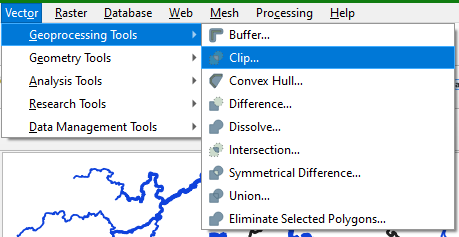
2. In the Clip dialogue choose channels as Input layer and Rur_catchment as Overlay layer. Name the Clipped result Rur_channels.shp.
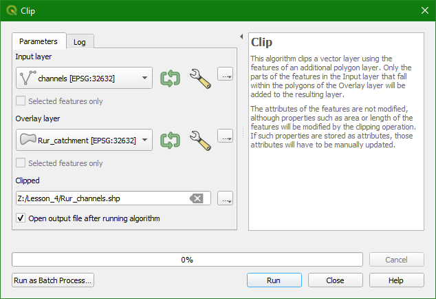
3. Click Run and click Close when the processing has finished.
4. Copy the style from channels and paste it to Rur_channels. Click right on the channels layer and choose Styles | Copy Style | All Style Categories. Then click right on Rur_channels and choose Styles | Paste Style | All Style Categories.
In a similar way we can clip the DEM to the catchment boundary.
5. From the main menu choose Raster | Extraction | Clip Raster by Mask Layer...
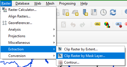
6. In the Clip Raster by Mask Layer dialogue choose DEM_clipped as Input layer. Use Rur_catchment as the Mask layer and use -9999 to Assign a specified nodata value to output bands. Also check the boxes to Match the extent of the clipped raster to the extent of the mask layer and Keep the resolution of input raster. Name the Clipped (mask) output Rur_DEM.
7. Click Run and click Close after processing.
8. Copy the style from DEM_clipped to Rur_DEM and also add the blending with hillshade in a similar way.
The result should now look like this:
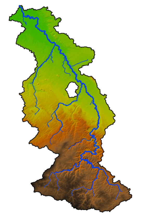
Note that we'll not use the Rur_DEM in the next section, because we are going to use a special styling technique to highlight the study area.
12. Styling the Resulting Catchment Area
To show the results of your analysis you can use a technique named Inverted Polygon Shapeburst Fills to focus attention on the Rur Catchment.
1. Open the Layer Styling panel by clicking the ![]() button. Set the target layer to Rur_Catchment.
button. Set the target layer to Rur_Catchment.
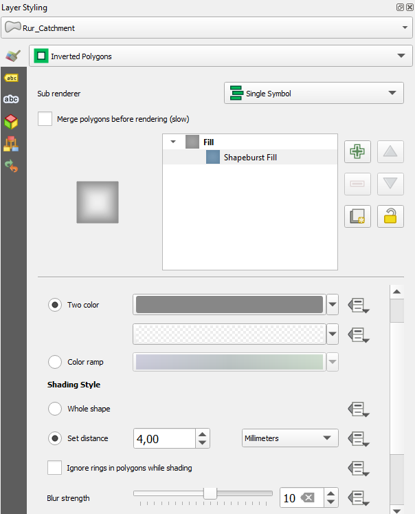
2. Change from a Single symbol renderer to an Inverted polygons renderer. This renders the data as the inverse of it's geometry, i.e. you'll style everything outside of the polygon. This creates a mask around the Rur valley.
3. Next select the Simple Fill component. Then change the Symbol layer type to Shapeburst fill. In the Gradient colors section use the default Two color method. Change the first color to an RGB value of 135 | 135 | 135. Change the second color to white with an opacity of 65%.
4. In the Shading style section, click the Set distance option and set the distance to 4 mm.
5. Increase the Blur strength to 10.
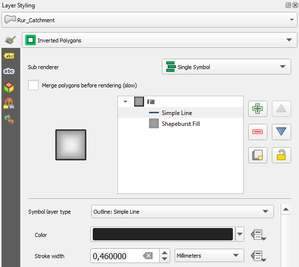
6. Finally at the top of the Layer Styling Panel select the Shapeburst fill component.
7. Click the Add symbol layer ![]() button. Change the new Simple fill renderer to a Symbol layer type of Outline: simple line. Give it a Color of black and a Stroke width of 0.46 mm.
button. Change the new Simple fill renderer to a Symbol layer type of Outline: simple line. Give it a Color of black and a Stroke width of 0.46 mm.
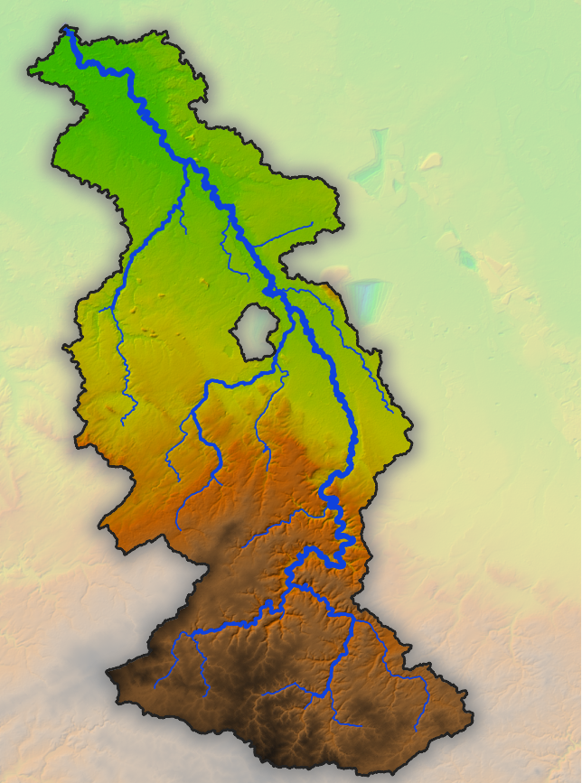
This gives us the nicely styled basin as shown in in the figure below. Note that the DEM on the picture is DEM_clipped with the corresponding hillshade. If we would have used the Rur_DEM layer (the one we have created in the previous section by clipping with the Rur_Catchment as mask layer), the inverted polygon shapeburst fill styling effect doesn't make sense. Clipping the DEM to the boundary is useful for further processing. For visualisation purposes and map design the inverted polygon shapeburst fill styling gives a nicer result.
13. Storing the Data in a GeoPackage
To keep the data together and enable easy distribution it is good to save the layers as a GeoPackage.
1. In the Processing Toolbox look for the Package Layers tool.
2. In the Package Layers dialogue click the ![]() and select all layers you want to add. Note that these are only the vector layers.
and select all layers you want to add. Note that these are only the vector layers.
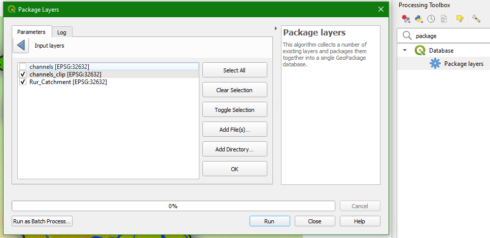
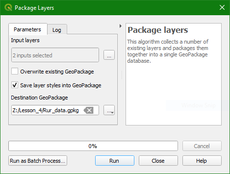
3. Save it as Rur_data.gpkg and click Run and Close when it's done. By default it will also save the styles.
4. We can add the raster layers from the Browser panel. Simply drag the raster layers (e.g. the DEM) to the Rur_data.gpkg. You might need to refresh the Browser panel to see the GeoPackage.
Finally, we can also save the project in the GeoPackage. In that way all data and settings are stored in one file that can be shared with others in a much easier way than separate shapefiles and styling files.
5. Add the layers from the GeoPackage to the project. Copy the styles of
the rasters if needed. Remove the layers that are not in the GeoPackage.
6. In the main menu choose Project | Save to | GeoPackage...
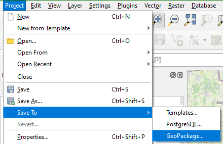
7. Choose for Connection Rur_data.gpkg and give the project a name, e.g. Rur
14. Conclusions
In this lesson you have learned to:
- find and download SRTM DEM tiles from the EarthExplorer website
- mosaic raster layers into a virtual raster
- reproject rasters
- create subsets of rasters
- fill sinks in a DEM
- calculate and style flow direction raster layers
- calculate Strahler orders
- delineate streams
- delineate catchments
- style layers for visualising catchments