Tutorial: Map Algebra with PCRaster Python
| Site: | OpenCourseWare for GIS |
| Course: | FOSS4G 2022 Workshop Hydrological analysis with PCRaster in QGIS and Python |
| Book: | Tutorial: Map Algebra with PCRaster Python |
| Printed by: | Guest user |
| Date: | Saturday, 27 June 2026, 12:41 AM |
1. Introduction
This tutorial will first present some theory on map algebra and will introduce the PCRaster Environmental Modelling Language.
The tutorial contains three Jupyter Notebook tutorials:
- Map algebra for finding inaccessible wells in a study area
- Interpolation of borehole data using Inverse Distance Weighting (IDW) and Thiessen methods
- Stream and catchment delineation
The first one will be run online. The other two will be run locally. You'll learn how to install the Anaconda distribution, create an environment with the necessary libraries and run Jupyter Notebooks from the Anaconda prompt.
After this module you'll be able to:
- Explain the concepts of map algebra
- Convert rasters using GDAL in Python
- Use PCRaster in Python for map algebra
- Use PCRaster for interpolations
- Use PCRaster for stream and catchment delineation
2. Theory
The PCRaster Environmental Modelling Language
The video below will introduce you to the PCRaster environmental modelling language.
More information about PCRaster can be found at: http://www.pcraster.eu. You can subscribe there to the PCRaster mailing list to read and post questions and answers to the community.
Theory of Map Algebra
Watch this lecture to learn more about Map Algebra in GIS:
3. Spatial Analysis with Map Algebra
Use the button below to run the PCRaster Map Algebra Jupyter Notebook in Binder:
![]()
If you are more experienced and want to run the Jupyter Notebook locally you can download it here:
https://github.com/jvdkwast/PCRasterTutorials (GitHub)
The data used in this tutorial is an artificial dataset.
This video shows the result of the Map Algebra tutorial:
4. Install Miniconda and Packages
For the next tutorials you need to install Miniconda and PCRaster on your computer and run the Jupyter Notebooks locally. You can use the instructions from the video above. Here are the steps:
2. Open Miniconda Prompt from the Windows Start Menu
3. Type:
conda create --name tutorials -c conda-forge pcraster qgis python=3.9 matplotlib jupyterlab pycrs numpy git
This will create a new environment with the name tutorials and will install the necessary libraries that we'll use.
4. Activate the new environment by typing
conda activate tutorials
5. Use the commands to go to the folder where you want to save the tutorials (note that the next step will create a subdirectory PCRasterTutorials there).
6. Go to https://github.com/jvdkwast/PCRasterTutorials
7. Click the Code button

8. Copy the HTTPS link
9. With git we can interact with git repositories such as GitHub. Run the following command:
git clone https://github.com/jvdkwast/PCRasterTutorials.git
This will download all the tutorial materials of this and the next module to the subdirectory PCRasterTutorials.
To run the tutorials go to the PCRasterTutorials subdirectory and run the command
jupyter lab
This will open your browser and you can choose the notebook.
This video shows the procedure:
5. Spatial interpolation of borehole data
To run the Jupyter Notebook of this tutorial make sure you have followed the instructions for installing Miniconda and downloading the tutorials in the previous unit. We assume that you're in the Miniconda prompt and that you're in the tutorials environment.
- Run the command from the PCRasterTutorials directory:
jupyter lab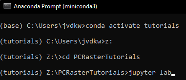
- Go to the subdirectory \PCRasterTutorials\GroundwaterInterpolation
- Click on Groundwater_level.ipynb so the Jupyter Notebook will open in a tab.
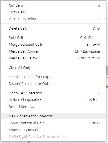
- Click right in the Jupyter Notebook and choose New Console for Notebook to add a Python Console that is linked to the notebook.
- Click the + next to the Groundwater_level.ipynb tab to add a Terminal, which you can use to navigate your file system with the CLI command that you've learned in Module 1.
- Arrange the tabs in such away (drag and drop) that your screen looks like this:
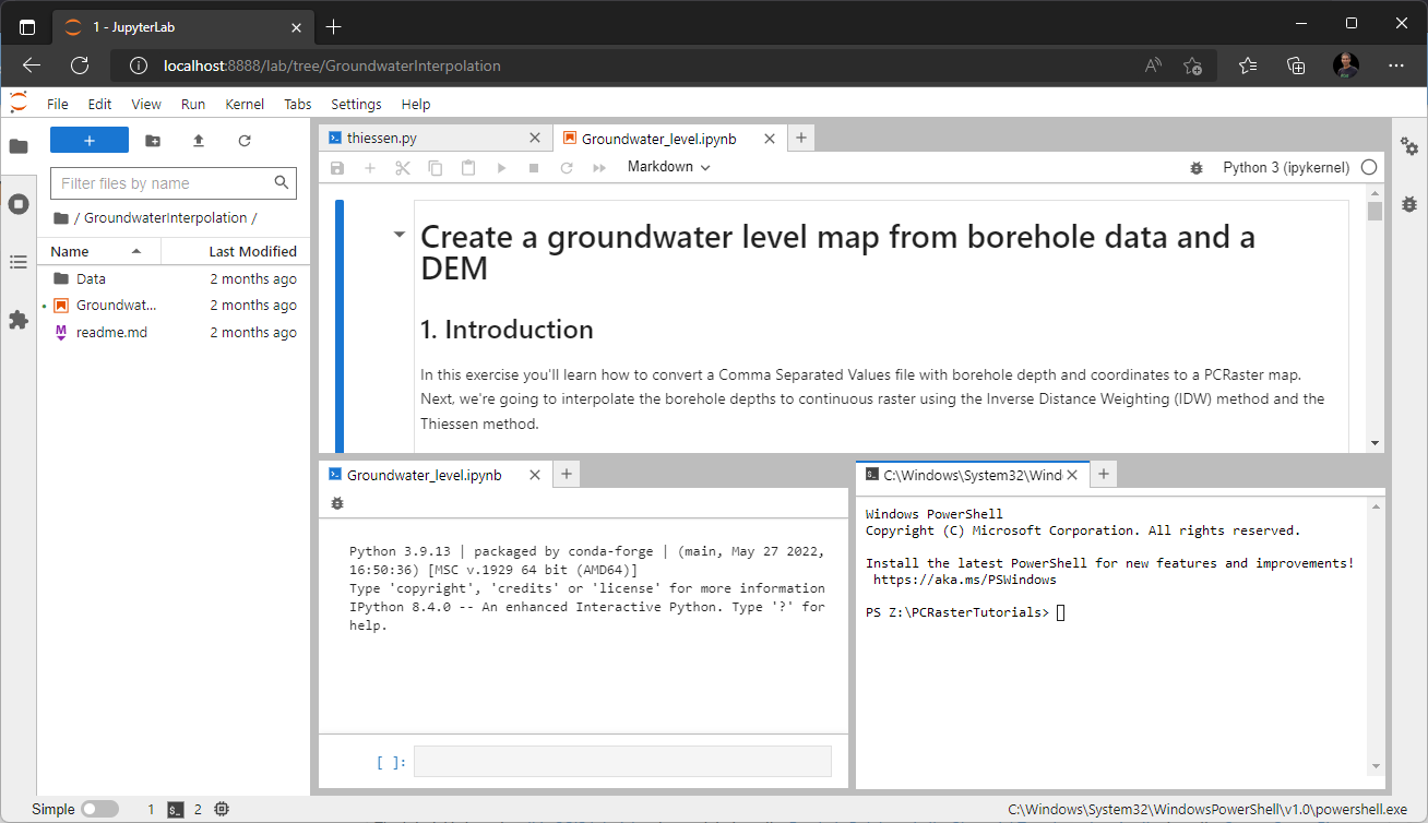
- Follow the tutorial in the Jupyter Notebook, use the Python Console to test code and use the Terminal to navigate the file system.
The tutorial is based on this QGIS tutorial and uses data from the Borehole Database in the Stampriet Transboundary Aquifer from the Orange-Senqu River Basin GIS Server. If you want to visualise the data and results in QGIS, the projection is EPSG:32734.
This video shows the whole exercise in the Jupyter Lab interface:
6. Stream and Catchment Delineation
To run the Jupyter Notebook of this tutorial make sure you have followed the instructions for installing Miniconda and downloading the tutorials as explained before. We assume that you're in the Miniconda prompt and that you're in the tutorials environment.
- Go to the subdirectory \PCRasterTutorials
- Run the command
jupyter lab - In Jupyter Lab browse to the PCRasterCatchmentDelineation folder, click on ContentsCatchmentDelineation.ipynb and follow the tutorial.
This tutorial uses data (included in the Data folder) from the Shuttle Radar Topography Mission: SRTM 1-Arc Second. If you want to apply it to other areas, you can download the data from USGS Earth Explorer.
You can write the code also in the QGIS Python Console. In that way it's easier to visualise the results. You can use QGIS from your miniconda environment or the standard QGIS on Windows if you have installed PCRaster through the OSGeo4W installer.
This video shows the exercise applied in the QGIS Python Console: