Tutorial: Create a groundwater level map from borehole data and a DEM
| Site: | OpenCourseWare for GIS |
| Course: | GIS training for Hydrogeological Applications |
| Book: | Tutorial: Create a groundwater level map from borehole data and a DEM |
| Printed by: | Guest user |
| Date: | Thursday, 16 July 2026, 10:19 AM |
Description
Table of contents
- 1. Introduction
- 2. Load a boreholes dataset from a GeoNode SDI
- 3. Export WFS data to GeoPackage
- 4. Select boreholes in a specific area
- 5. Calculate the borehole density
- 6. Download the SRTM 1-Arc Second DEM
- 7. Clip and reproject the DEM
- 8. Style the DEM
- 9. Sample DEM elevation at boreholes
- 10. Compare reported elevation with DEM values
- 11. Replace nodata values with DEM elevation
- 12. Calculate the groundwater level in the boreholes
- 13. Interpolate groundwater levels in boreholes to a raster
- 14. Derive groundwater contours
1. Introduction
After this tutorial you'll be able to:
- Load a borehole/wells dataset from an SDI into QGIS
- Calculate the density of the boreholes in a polygon
- Download the SRTM 1-Arc Second DEM
- Clip and reproject a DEM
- Style a DEM
- Sample elevation at the borehole location and compare it with the elevation attribute
- Make corrections and calculations in the attribute table
- Interpolate groundwater levels of the boreholes to a raster
- Create and visualise contour lines
2. Load a boreholes dataset from a GeoNode SDI
We'll start with loading a boreholes dataset from a GeoNode SDI to QGIS.
In this tutorial we'll use the Borehole Database in the Stampriet Transboundary Aquifer from the Orange-Senqu River Basin GIS Server, which is a GeoNode SDI.
1. Check the metadata of the Borehole Database in the Stampriet Transboundary Aquifer. Read the info tab and check the attributes that are in the layer.

2. Start QGIS with an empty project.
3. Click the Open Data Source Manager button  in the toolbar.
4. Choose the GeoNode tab.

5. Click the New button to create a new service connection.
6. In the Create a New GeoNode Connection dialogue type ORASECOM for the Name and copy the URL http://gis.orasecom.org.

7. Click Test Connection.
If the test is successful you'll see this popup:

If the connection fails, check your internet connection and the URL.
8. Click OK to close the popup.
9. Click OK in the dialogue to close it and the new connection is added.
10. Click the Connect button.
If you'll get an error in a popup that you can ignore. Click OK to remove the error message.

Then you'll see the layers on the GeoNode listed.
We're going to use data from the Stampriet aquifer.
11. Type stampriet at filter.

12. Click stasboreholes WFS layer (indicated in the figure above).
We use a WFS Web service, because we want to access the data and not just a picture like with WMS data.
13. Click Add to add the layer to the map canvas.
14. Click Close to close the dialogue.
It will take a while to load from the internet.

Just wait until loading has completed. Then you'll see this:

In the next section we're going save this WFS layer to a GeoPackage to further use locally.
3. Export WFS data to GeoPackage
Our borehole dataset is still in the WFS format and in a Geographic Coordinate System (GCS) with coordinates in degrees latitude/longitude. For our purpose of interpolating elevation, we need to store the file locally and reproject it to UTM Zone 34S/WGS-84.
1. In the Layers panel click right on the geonode:stasboreholes layer.
2. Choose Export | Save features as...

3. In the Save Vector Layer as... dialogue choose GeoPackage as the Format. Click the  button to browse to a folder on your harddisk where you want to store the GeoPackage (e.g. Z:\Stampriet). Name it Stampriet_Data.gpkg. Type for Layer name Boreholes.

4. Click the  button to change the projection of the output layer.
5. In the Coordinate Reference System Selector dialogue type 32734 (that's the EPSG code) at Filter to search for the WGS 84 / UTM Zone 34S projection. Click on the projection name and click OK to return to the dialogue window.

6. Click OK to perform the export.
7. After the Stampriet_Data Boreholes layer has been added to the map canvas, remove the geonode:stasboreholes layer by clicking right on it and choose Remove layer.... Confirm with OK.
Now we have a local copy of the boreholes layer.
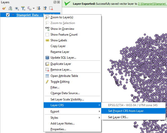
8. Change the OTF projection of the project: in the Layers panel click right on Stampriet_Data Boreholes and choose Set CRS | Set Project CRS from Layer
9. Save the project in the GeoPackage. Call it Strampriet.
In the next section we're going select the boreholes in a specific area.
4. Select boreholes in a specific area
For this tutorial we're only interested in the boreholes in the area around Stampriet.
An imaginary boundary polygon is provided in the tutorial data.
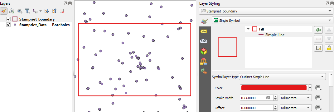
1. Add the Stampriet_boundary shapefile to the project.
2. In the Layers panel click right on Stampriet_boundary and choose Zoom to layer.

3. Style the boundary with a red outline.
Now we're going to clip the boreholes that fall within the boundary and save it to our GeoPackage.
4. From the main menu choose Vector | Clip...

5. In the Clip dialogue choose Stampriet_Data Boreholes as Input layer and Stampriet_boundary as Overlay layer. Save the Clipped result to the Stampriet_Data GeoPackage with the layer name boreholes_clipped.

6. Click Run. Click Close to close the dialogue after processing.
7. Remove the Stampriet_Data Boreholes layer from the Layers panel.

In the next section we'll calculate the density of boreholes in this area.
5. Calculate the borehole density
Now we have the boreholes within a study area (this could also be an aquifer) we can calculate the borehole density.
1. Open the Processing Toolbox: in the main menu go to Processing | Toolbox.
2. In the Processing Toolbox choose Vector analysis | Count points in polygon.

3. In the Count Points in Polygon dialogue choose Stampriet_boundary as Polygons and boreholes_clipped as Points. Change the Count field name to No of boreholes. Save the Count output to the Stampriet_Data GeoPackage with the layer name Stampriet study area.
We're
using that output name, because this tool makes a copy of the
Stampriet_boundary polygon and adds the No of boreholes field. We didn't
have the study area boundary yet in our GeoPackage, so now we'll add it
in this way.

4. Click Run. Click Close after processing.
Note that if your input has multiple polygons (e.g. different aquifers) it will produce the count per polygon. You can apply the next steps then to calculate the borehole density for all polygons.
5. Copy the style of Stampriet_boundary to Stampriet study area: in the Layers panel click right on Stampriet_boundary and choose Styles | Copy Style | All Style Categories. Then click right on Stampriet study area and choose Styles | Paste Style | All Style Categories.
6. Remove the Stampriet_boundary from the Layers panel.
Now let's have a look at the Stampriet study area attribute table.
7. In the Layers panel click right on Stampriet study area and choose Open Attribute Table.
You can see that we have 64 boreholes in the study area.

Now we need to calculate the area of the study area polygon.
8. In the attribute table click the  button to toggle editing on.
9. Click  to open the Field calculator.
10. In the Field Calculator dialogue Create a new field with the Output field name Area (km2) and Output field type Decimal number (real).
11. Under Expression choose from the functions in the middle panel Geometry | $area and double click on $area to add it to the expression. $area calculates the area of the polygon in map units. In our case that's m2. Complete the expression so it states:
$area / 1000000
Use the  button to add the division.

The result should look like the figure below.

The next step is to calculate the borehole density.
13. Click to open the Field calculator.
14. In the Field Calculator dialogue Create a new field with the Output field name Borehole density per km2 and Output field type Decimal number (real). Under Expression with the following equation:
"No of boreholes" / "Area (km2)"
Remember you can add the fields by double clicking the field names under Fields and values in the middle panel. Use the button to add the division.

16. Toggle off editing by clicking and click Save in the popup to save the results.
We have calculated that the borehole density in the study area is 0.2 per km2.

In the next section we're going to add a DEM to the project.
6. Download the SRTM 1-Arc Second DEM
In this section we're going to add a DEM to the project. We'll use the Shuttle Radar Topography Mission (SRTM) 1 Arc Second product. This is a free DEM that covers 56°S to 60°N and has a spatial resolution of approximately 30 m on the equator.
You can download the SRTM tiles from the USGS Earth Explorer website or through a plugin. Here we're going to use the SRTM Downloader plugin in QGIS.
1. In the main menu go to Plugins | Manage and Install Plugins...

2. Look for the SRTM-Downloader plugin, install the plugin and return to the project.

3. In the toolbar click this button to open the SRTM-Downloader dialogue  .
.
4. In the SRTM-Downloader dialogue click Set canvas extent (make sure you're still zoomed to the boundary of the study area!). For the Output-path browse to the folder where the data for this project is stored.

5. Click Download.
6. The first time a popup will promt for the Login information. In order to download the SRTM tiles you need to make an account at https://urs.earthdata.nasa.gov/users/new.

7. Fill in your Username and Password. Click Save Credentials and click OK.
Now it will start downloading the SRTM tile that covers the study area.
8. Click OK in the popup.

9. Close the dialogue.

7. Clip and reproject the DEM
The SRTM tile is added to the map canvas. If you zoom to the S25E018.hgt layer you can see that it covers a much larger area. Also the projection is in Geographic Coordinate System (GCS) with latitude/longitude coordinates in degrees (EPSG:4326).
So we have to clip and reproject the DEM and add it to our GeoPackage.
1. In the Layers panel click right on S25E018.hgt and choose Export | Save As...


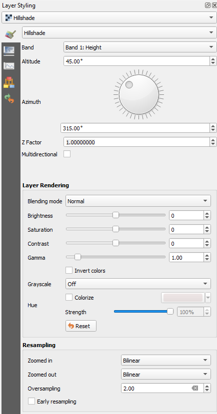
8. Style the DEM

 to open the Layer Styling panel.


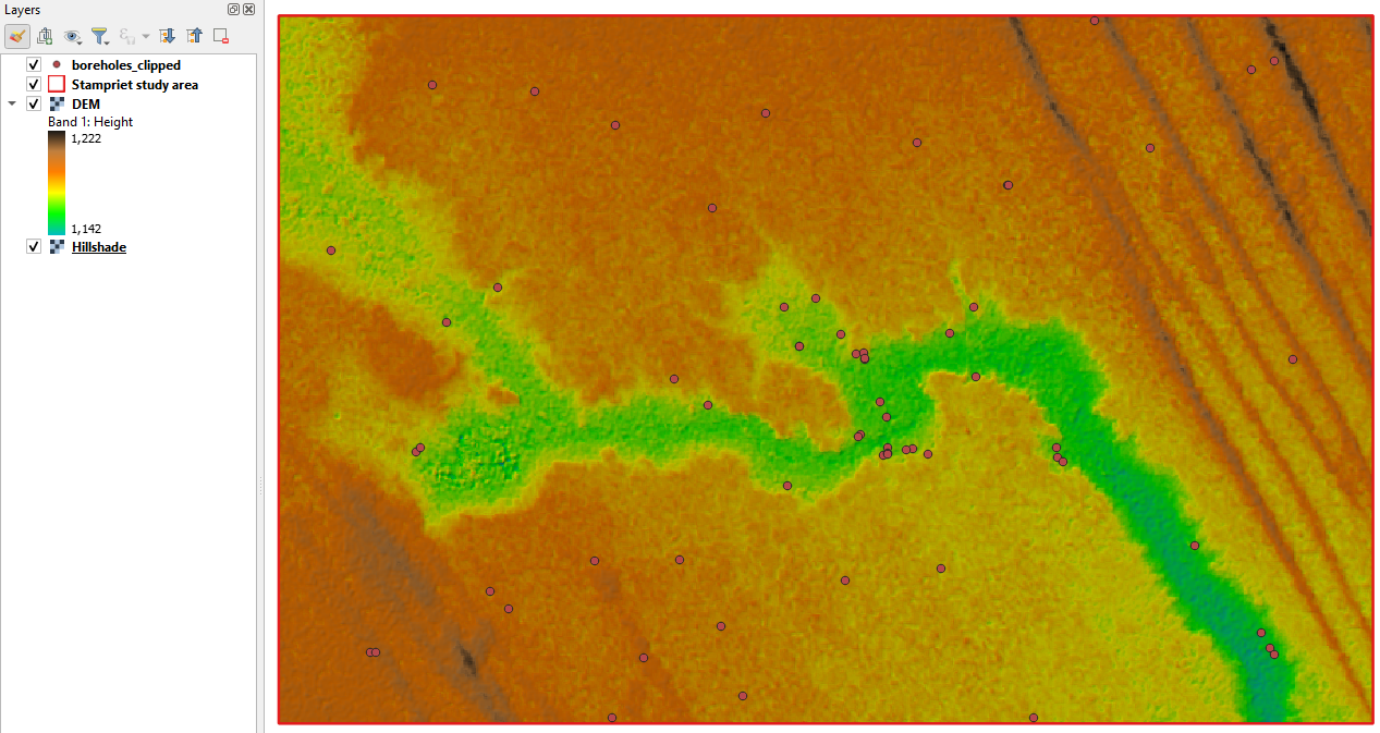
Now your project should look like the figure below.
In the next section we're going to add the DEM elevations to the attribute table of the boreholes.
9. Sample DEM elevation at boreholes
We're now going to sample the DEM elevations at the borehole locations.
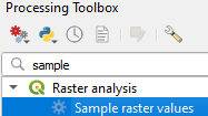
1. In the Processing Toolbox choose go to Raster analysis | Sample raster values
2. In the dialogue choose boreholes_clipped as Input layer and DEM as Raster layer. For Output column prefix type Z_. Save the Sampled output layer to the GeoPackage with the name Boreholes_Z.
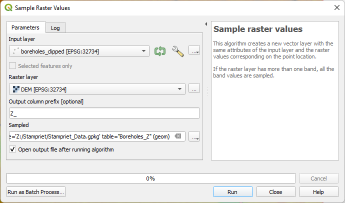
3. Click Run. Click Close to close the dialogue after processing.
4. Check the attribute table of the Boreholes_Z layer.
You can see that the Z_1 field has been added.
In the next section we're going to create a scatter plot of the reported elevation and the Z value from the DEM.
Note that if you want to sample values from multiple vectors and rasters you need to use the Point Sampling Tool plugin, which was used in the video.
10. Compare reported elevation with DEM values
In the Boreholes_Z attribute table we have the reported elevation and the values from the DEM. Let's compare the two fields by making a scatter plot.
The elevation field contains a lot of no data values. Let's not consider those for the scatter plot.
1. Open the attribute table of Boreholes_Z.
2. Click the Select by attributes button  .
.
3. Write the expression
"elevation" < 0

4. Click Select Features and click Close to close the dialogue.
10 features have been selected. We could remove them from the attribute table by toggling to editing mode and click the trash bin. For the scatter plot, however, we can invert the selection and indicate we only want to use the selected features.
5. Click  to invert the selection.
To make the scatter plot we need to install the Data Plotly plugin.
6. Install the Data Plotly plugin from the Plugins manager.

7. Click the  icon in the toolbar to open the Data Plotly panel.
8. In the Data Plotly panel choose Scatter Plot as Plot type. Choose Boreholes_Z as Layer. Check the box to Use only selected features. Choose elevation for the X field and Z for the Y field. Keep the styling as default.

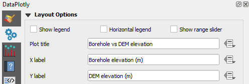
9. Click  to go to legend configuration tab.
10. Uncheck the Show legend box. Change the Plot title to Borehole vs DEM elevation. Write Borehole elevation (m) for the X label and DEM elevation (m) for the Y label. Keep the rest as default.
11. Click Create Plot at the bottom of the panel.
Check the plot.

In the next section we're going to replace the missing values of elevation with the DEM elevations.
11. Replace nodata values with DEM elevation
Because the scatter plot looks reasonable, we're going to replace the nodata values in the elevation field of the Boreholes_Z.shp layer with the values from the DEM.
1. Open the attribute table from Boreholes_Z layer.
2. Click  to deselect all.
3. Click  to toggle to editing mode.
4. Change the output to elevation and click the  button to build the expression.

5. In the Expression dialogue build the following expression:
if( "elevation" < 0, "Z_1" , "elevation" )
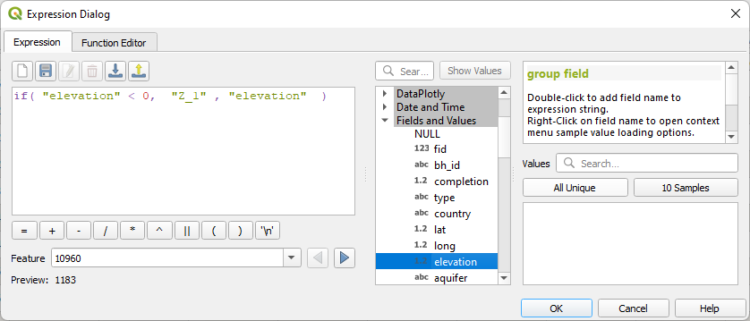
This means: if the elevation field has values less than zero, then use the Z field values, else use the elevation field values.
6. Click OK.
The expression should now look like this in the attribute table:
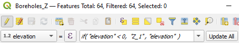
7. Click Update All.
Now all missing values have been replaced with the elevation from the DEM.
8. Click to to toggle off editing and click Save to save the results.
In the next section we're going to calculate the absolute groundwater levels in the boreholes.
12. Calculate the groundwater level in the boreholes
In the attribute table of the boreholes we have the depth to the water table.
In this section we're going to calculate the absolute elevation of the water level in the boreholes.
1. Open the attribute table of Boreholes_Z.
2. Click  to toggle to editing mode.
First we're going to delete the features with missing data for depth in the depth_m field.
3. Click  to open the Select features using an expression dialogue.
4. Build the following expression
"depth_m" < 0

5. Click Select Features. Click Close to close the dialogue.
6. Click  to delete the selected features.
7. Click  to save the edits until now.
8. Click  to open the Field calculator dialogue.
9. In the Field Calculator dialogue Create a new field with the Output field name GW_level_m and Output field type Decimal number (real). Keep the other settings as default and type the following expression:
"elevation" - "depth_m"
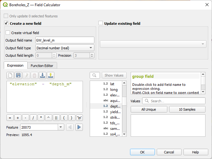
10. Click OK.
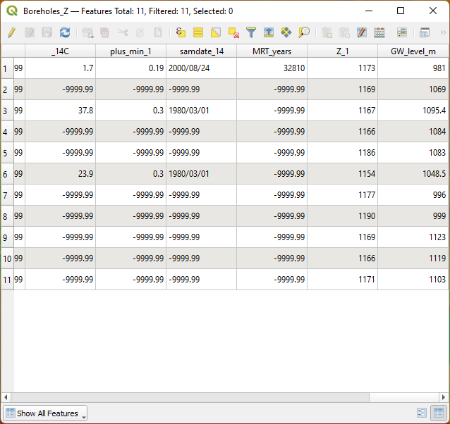
11. Check the results and click to toggle off editing. Click Save to save the results.
13. Interpolate groundwater levels in boreholes to a raster
Now we have the groundwater levels in the boreholes we can interpolate the points to a raster.
We're going to use two methods: Inverse Distance Weighting (IDW) and Thiessen polygons.
Let's start with the IDW interpolation.
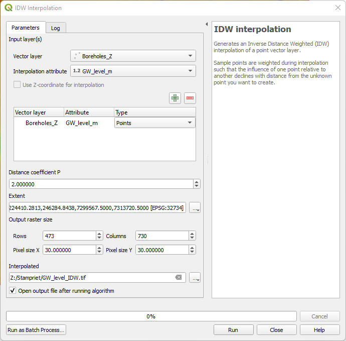
1. In the Processing Toolbox choose Interpolation | IDW interpolation.

2. In the IDW Interpolation dialogue choose the Boreholes_Z layer as Vector layer. Use the GW_level_m as Interpolation attribute. Click  to add these settings to the list. Keep the Distance coefficient P at 2 for an exponential decay function. Select the Extent from the Stampriet study area layer. Change the Pixel size to 30 m. Save the Intepolated raster to the project folder as GW_level_IDW.tif.
3. Click Run. Click Close after processing.
Let's style the result with a colour ramp.
4. Select the GW_level_IDW layer in the Layers panel and click  to open the Layer Styling panel.
5. In the Layer Styling panel change the renderer to Singleband pseudocolor and choose All Color Ramps | RdBu

The Layer Styling panel should now look like this.

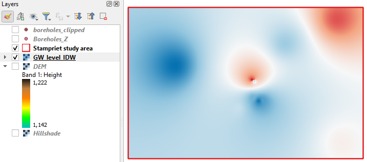
And
the interpolated layer should look like the figure below. You can play
with different ramps and classes to improve the visualisation. You can
see the the IDW interpolator creates a smooth output, but because the
amount of boreholes is low there's a lot of bias towards individual
boreholes and outliers.
Let's apply the Thiessen polygon (aka nearest neighbour or Voronoi tesselation) method now.
6. In the main menu choose Raster | Analysis | Grid (Nearest Neighbor).

7. In the Grid (Nearest Neighbor) dialogue choose the Boreholes_Z layer as Point layer. Under Advanced choose GW_level_m as Z value from field. Save the Interpolated (Nearest Neighbor) output to GW_level_Thiessen.tif. Keep the rest as default.
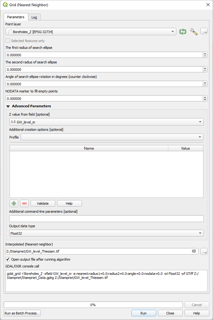
8. Click Run. Click Close to close the dialogue.
9. Style the result by copying the style from the IDW layer.
This
algorithm doesn't cover the whole study area but is limited to the so
called convex hull of the input point layer. It gives a less smooth
result then the IDW intepolation. However, with scarce data the nearest
value might be the best approximation.

In the next section we'll derive contour lines.
Note that if you want to use Thiessen polygons with control of the output extent and resolution, you can do this by adding GDAL options in the dialogue. Watch this video (optional) to see how this works:
14. Derive groundwater contours
We'll continue with the IDW result and will add contour lines.
An easy and quick way to visualise contour lines is to use the Contours renderer in the Layer Styling panel.
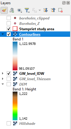
1. Make sure that the GW_level_IDW layer is completely visible in the map canvas.
2. Duplicate the layer, rename it to Contourlines and drag it above the GW_Level_IDW layer. Also check the box to make the layer visible.
2. In the Layer Styling panel change the renderer from Singleband pseudocolor to Contours.
3. Change the Contour Interval to 5 m and the Index Contour Interval to 25 m. Change the Contour Symbol to gray.
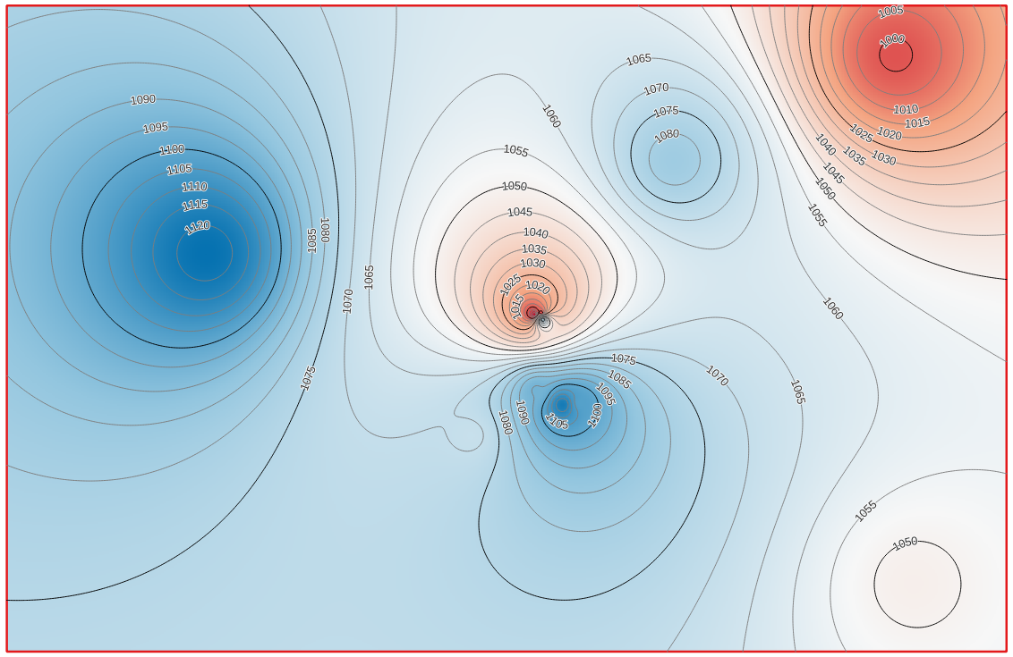
The map canvas should now look like this:
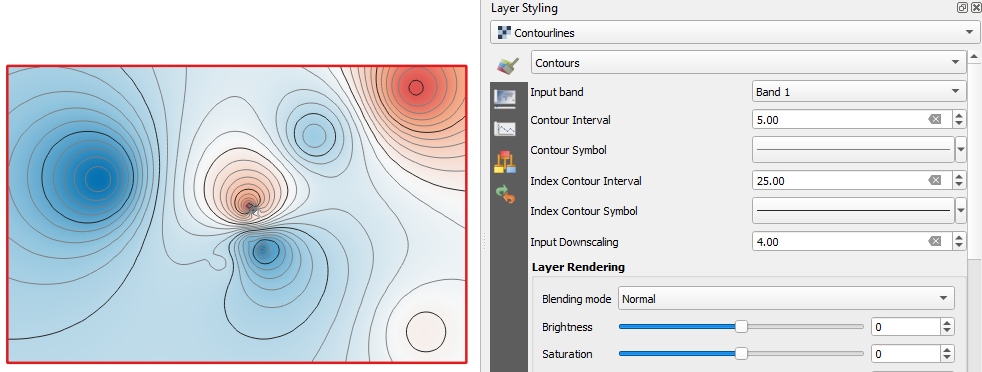
With the Input Downscaling setting you can change the smoothness of the lines. In this case the default is already smooth.
This is nice for visualisation, but not for calculations. Furthermore, we miss the labels with values of the contour lines. So, let's create a layer with contour lines.
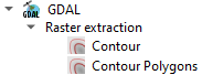
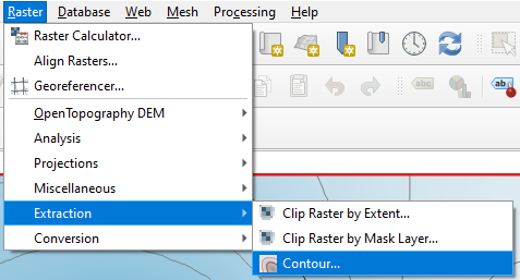
4. Choose from the main menu Raster | Extraction | Contour....
5. Choose the GW_level_IDW as Input layer, change the Interval between contour lines to 5 m. Set the Attribute name to Z. Keep the rest as default and save the result as a shapefile with the name contours.shp. Note that you can't save the layer into an existing GeoPackage.
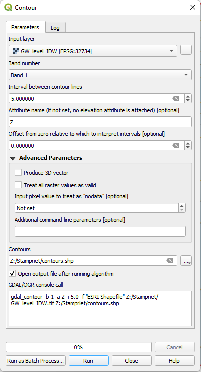
6. Click Run. Click Close after processing.
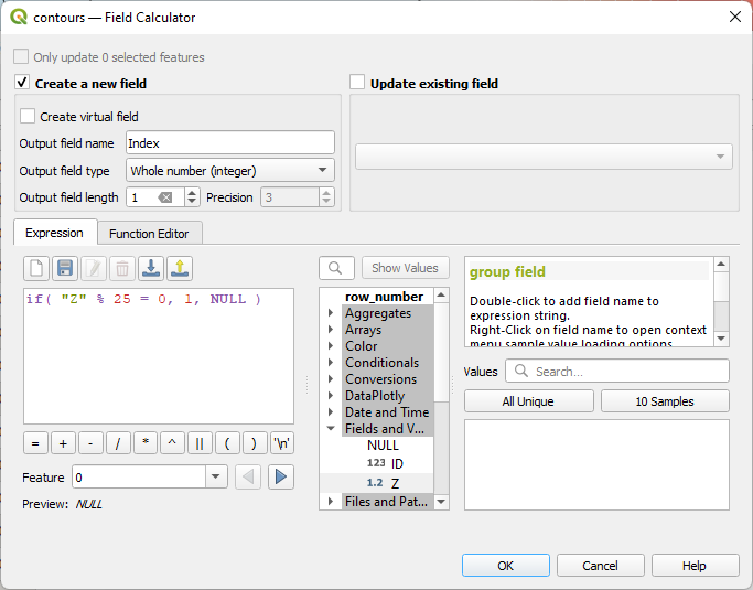
Let's style the calculated contour lines in the same way as the rendered lines.
if( "Z" % 25 = 0, 1, NULL )
 tab.
tab. tab. Change the Mode to Curved, check the On line box and uncheck the Above line box.
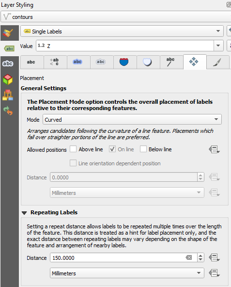
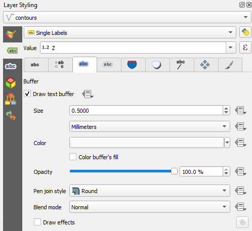
 tab. Check the box to Draw text buffer and set it to 0.5 mm. This makes the labels more readable through the contour lines.