Tutorial: Create a groundwater quality map from borehole data
| Site: | OpenCourseWare for GIS |
| Course: | GIS training for Hydrogeological Applications |
| Book: | Tutorial: Create a groundwater quality map from borehole data |
| Printed by: | Guest user |
| Date: | Sunday, 26 July 2026, 12:54 PM |
Description
1. Introduction
After this tutorial you'll be able to:
- Load a borehole/wells dataset from an SDI into QGIS
- Interpolate water quality attributes of the boreholes to a raster using
- Thiessen polygons
- Inverse Distance Weighting (IDW)
- Kriging
- Create and visualise contour lines
2. Load a boreholes dataset from a GeoNode SDI
We'll start with loading a boreholes dataset from a GeoNode SDI to QGIS.
In this tutorial we'll use the Borehole Database in the Stampriet Transboundary Aquifer from the Orange-Senqu River Basin GIS Server, which is a GeoNode SDI.
1. Check the metadata of the Borehole Database in the Stampriet Transboundary Aquifer. Read the info tab and check the attributes that are in the layer.

2. Start QGIS with an empty project.
3. Click the Open Data Source Manager button  in the toolbar.
4. Choose the GeoNode tab.

5. Click the New button to create a new service connection.
6. In the Create a New GeoNode Connection dialogue type ORASECOM for the Name and copy the URL http://gis.orasecom.org.

7. Click Test Connection.
If the test is successful you'll see this popup:

If the connection fails, check your internet connection and the URL. You can also try to continue and see if the layers are shown when you click Connect.
8. Click OK to close the popup.
9. Click OK in the dialogue to close it and the new connection is added.
10. Click the Connect button.
If you'll get an error in a popup that you can ignore. Click OK to remove the error message.

Then you'll see the layers on the GeoNode listed.
We're going to use data from the Stampriet aquifer.
11. Type stampriet at filter.

12. Click stasboreholes WFS layer (indicated in the figure above).
We use a WFS Web service, because we want to access the data and not just a picture like with WMS data.
13. Click Add to add the layer to the map canvas.
14. Click Close to close the dialogue.
It will take a while to load from the internet.

Just wait until loading has completed. Then you'll see this:

To check if the location of the boreholes makes sense we'll add a backdrop from OpenStreetMap.
15. Go to the Browser panel, expand XYZ Tiles and drag the OpenStreetMap layer to the map canvas. Make sure that the point layer is on top.
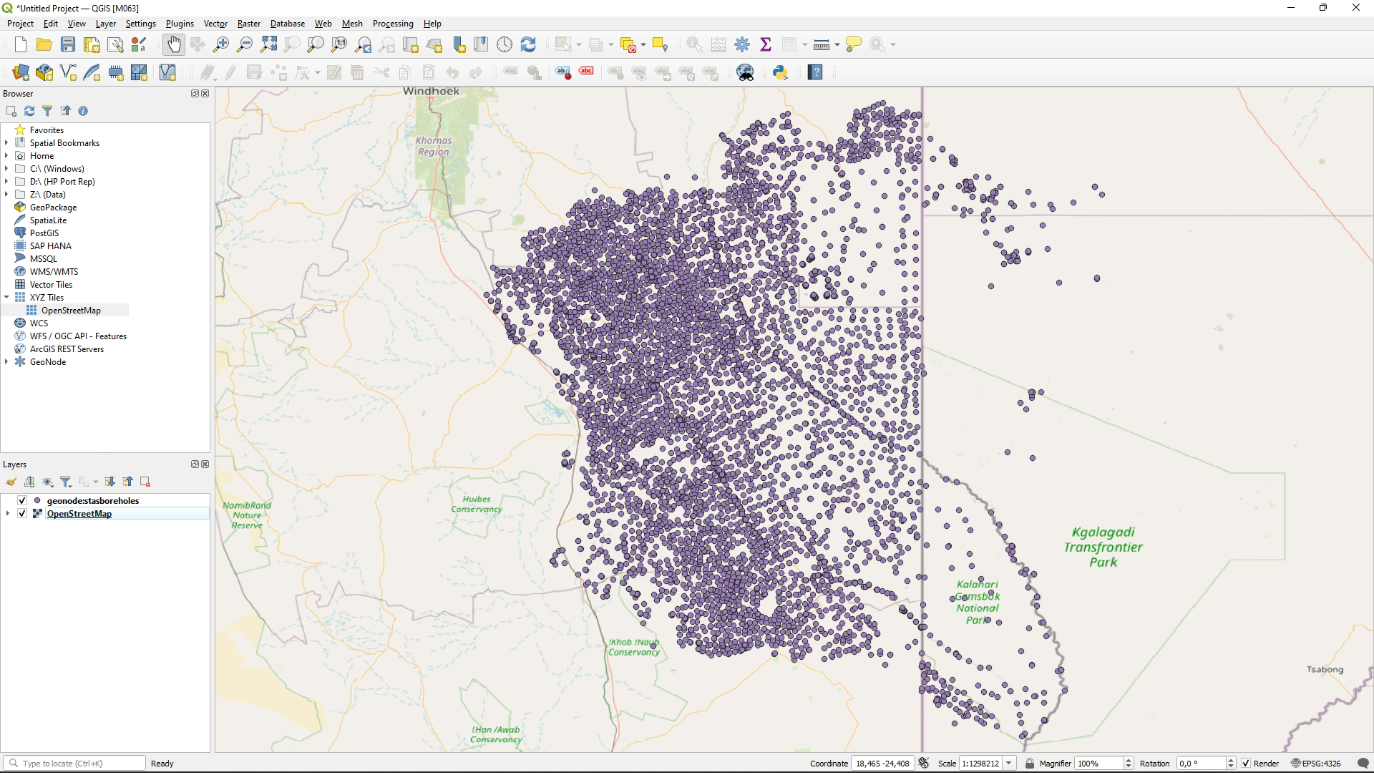
This looks correct.
In the next section we're going save this WFS layer to a GeoPackage to further use locally.
3. Export WFS data to GeoPackage
Our borehole dataset is still in the WFS format and in a Geographic Coordinate System (GCS) with coordinates in degrees latitude/longitude. For our purpose of interpolating elevation, we need to store the file locally and reproject it to UTM Zone 34S/WGS-84.
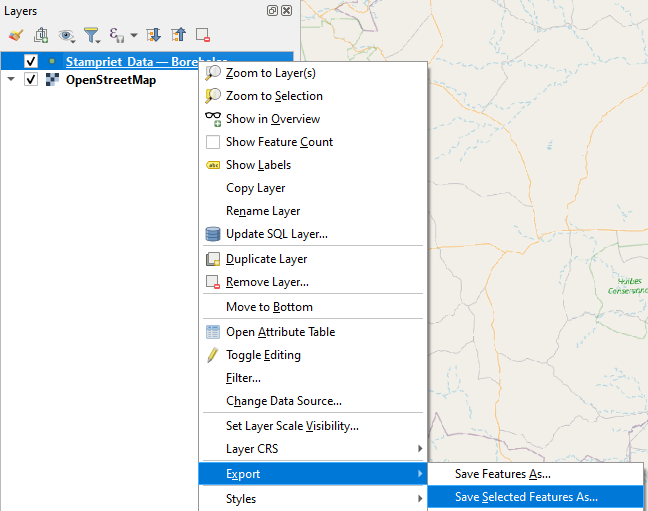
1. In the Layers panel click right on the geonode:stasboreholes layer.
2. Choose Export | Save features as...

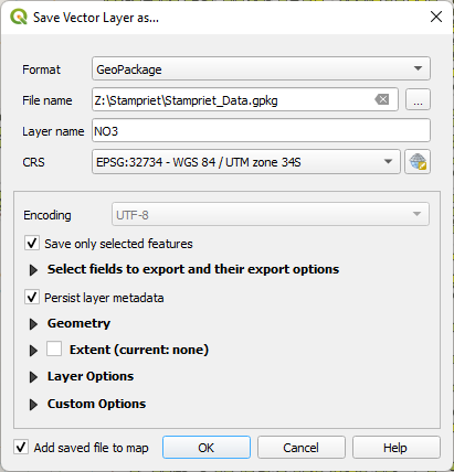
3. In the Save Vector Layer as... dialogue choose GeoPackage as the Format. Click the  button to browse to a folder on your harddisk where you want to store the GeoPackage (e.g. Z:\Stampriet). Name it Stampriet_Data.gpkg. Type for Layer name Boreholes.

4. Click the  button to change the projection of the output layer.
5. In the Coordinate Reference System Selector dialogue type 32734 (that's the EPSG code) at Filter to search for the WGS 84 / UTM Zone 34S projection. Click on the projection name and click OK to return to the dialogue window.

6. Click OK to perform the export.
7. After the Stampriet_Data Boreholes layer has been added to the map canvas, remove the geonode:stasboreholes layer by clicking right on it and choose Remove layer.... Confirm with OK.
Now we have a local copy of the boreholes layer.
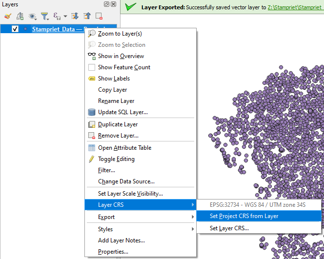
8. Change the OTF projection of the project: in the Layers panel click right on Stampriet_Data Boreholes and choose Set CRS | Set Project CRS from Layer
9. Save the project in the GeoPackage. Call it Stampriet.
In the next section we're going to interpolate the NO3 values of the boreholes data.
4. Interpolate groundwater quality data
In this chapter, we're going to interpolate water quality data. We'll use the NO3 attribute from our boreholes and interpolate the points to raster using:
- Thiessen polygons
- Inverse Distance Weighting (IDW)
- Kriging
4.1. Data preparation
Before we can interpolate the NO3 concentrations we need to remove missing values. Missing values can be NULL values in the attribute table or a specific out of range value.
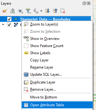
1. Let's inspect the attribute table. In the Layers panel right-click on the Boreholes layer and choose Open Attribute Table from the context menu.
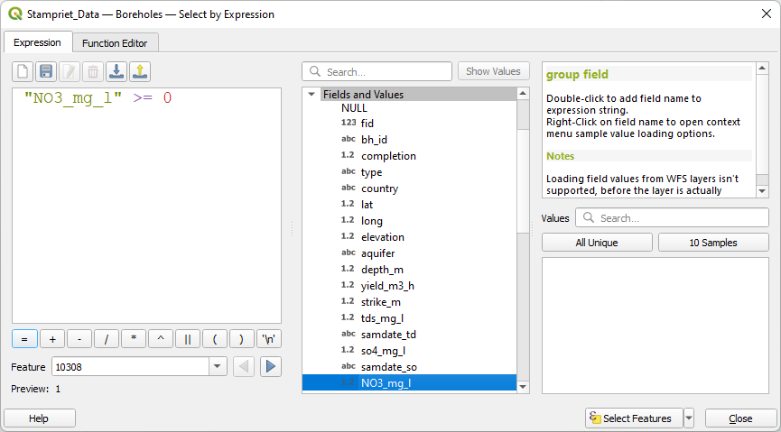
- Check the NO3_mg_l field. What is used here to indicate missing values?
 icon from the toolbar in the attribute table.
"NO3_mg_l" >= 0
4.2. Thiessen polygons
The first interpolation method that we'll use is the Thiessen method. It's also known as Voronoi tesselation or nearest neighbour interpolation. It will assign the closest know value to locations without measurements. When the point density is low and you don't have any knowledge of trends, this method is preferred.
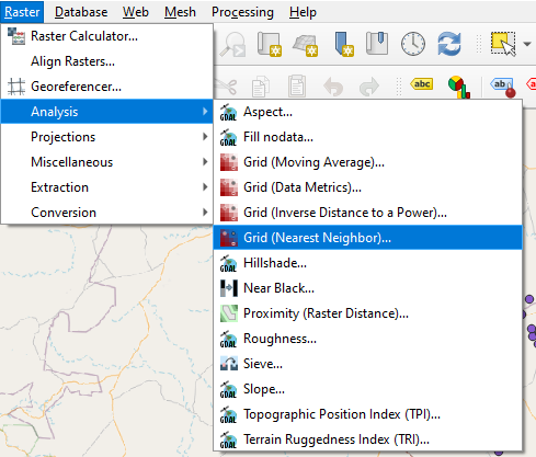
1. In the main menu of QGIS choose Raster | Analysis | Grid (Nearest Neigbor)....
2. In the Grid (Nearest Neighbor) dialog choose NO3 as the Point layer. At NODATA marker to fill empty points type -9999, otherwise it would use zeros, which are also values in our data. Scroll down and expand the Advanced Parameters section by clicking on the arrow. There choose the NO3_mg_l field at Z value from field. Keep the rest at default and save the result to NO3_Thiessen.tif in the same folder where you have the GeoPackage of this tutorial.
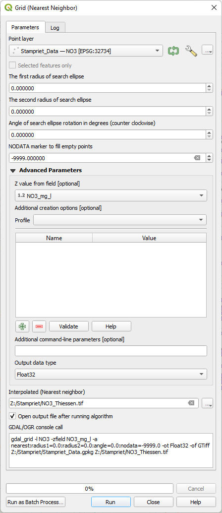
3. Click Run. Click Close after the processing has finished.
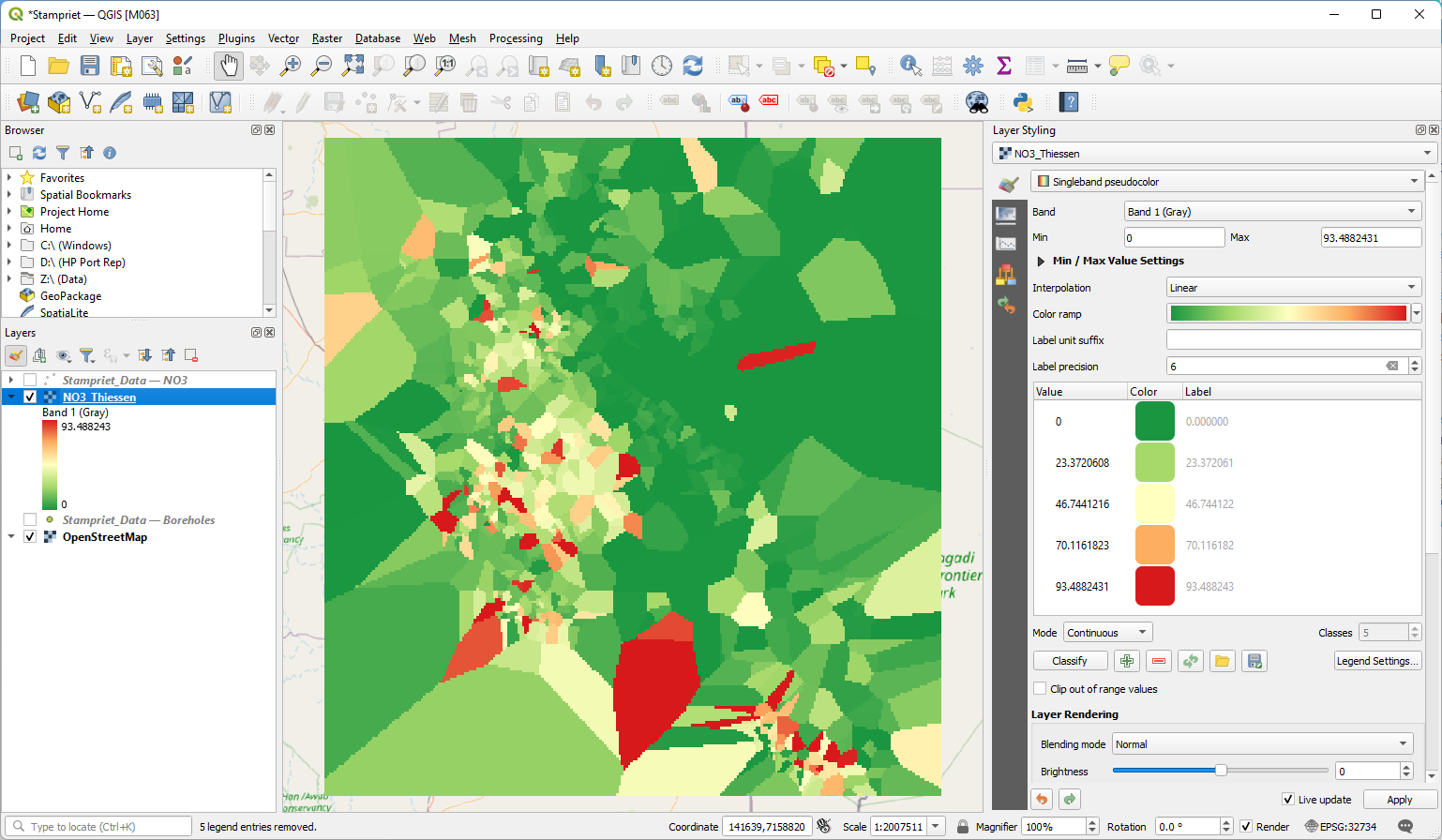
4. Change the styling of the Thiessen raster in the Layer Styling panel. Use Singleband pseudocolor, because it is a continuous raster (decimals), although it looks discrete. Choose a color ramp that is intuitive for this data.
The result should look like this:
In the next section we'll use the IDW interpolation method.
4.3. Inverse Distance Weighting
In this section we'll use the Inverse Distance Weighting (IDW) interpolation method. This method uses by default an exponential decay function for the weight of measurements as function of distance to the measurements. This works well with a high density of points.
You can find the IDW tool under Raster | Analysis | Grid (Inverse Distance to a Power)..., but we're going to use a similar tool from the Processing Toolbox, because there we can control the extent and spatial resolution of the raster output layer.
1. You can open the Processing Toolbox panel by clicking the gear  icon in the toolbar.
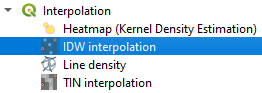
2. In the Processing Toolbox choose Interpolation | IDW interpolation.
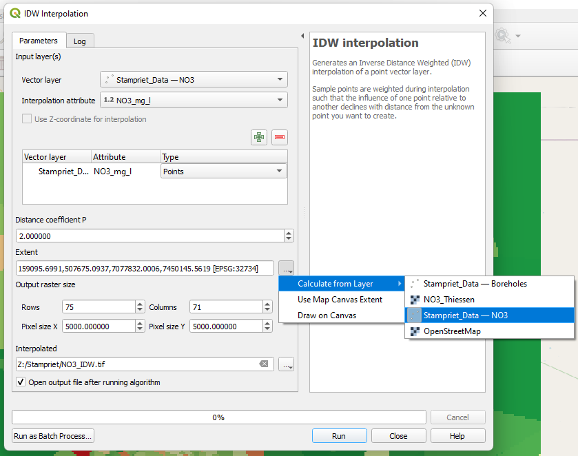
3. In the IDW Interpolation dialog choose the NO3 layer as Input layer and the NO3_mg_l field as Interpolation attribute. Click the  icon to add the points. Keep the Distance coefficient P at 2 for an exponential function. For Extent, use the dropdown menu to point to the extent of the NO3 point layer. Change the pixel size to 5000 m and save the result to NO3_IDW.tif.
4. Click Run. Click Close after processing.
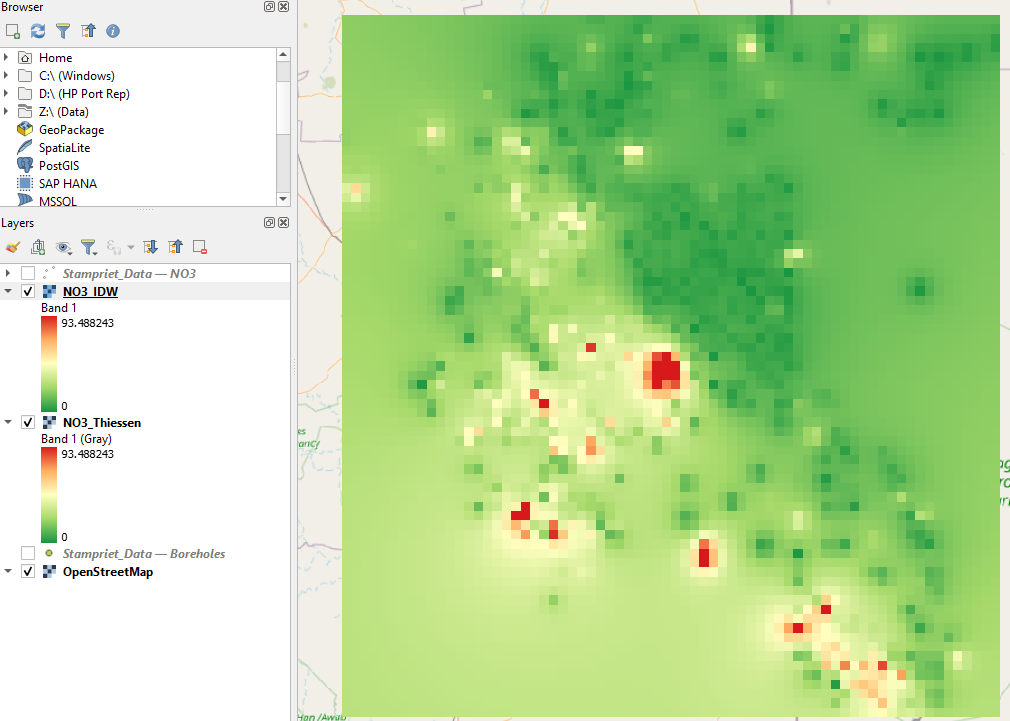
5. Copy the style from the Thiessen result to the IDW raster so they can be compared. You can do this easily by right-clicking on the Thiessen layer and choose Styles | Copy Style from the context menu. Then choose Styles | Paste Style for the IDW layer.
The result for IDW should look like this:
In the next section we'll use kriging as interpolation method.
4.4. Kriging
In this section we'll apply the kriging method for interpolating the NO3 measurements in our borehole dataset. Kriging uses the spatial autocorrelation in the dataset for interpolation. There are many different types of kriging, but here we use the most simple from: Ordinary Kriging. The method needs a semivariogram. With the Smart-Map plugin we can generate the semivariogram and fit models that can be used for kriging.
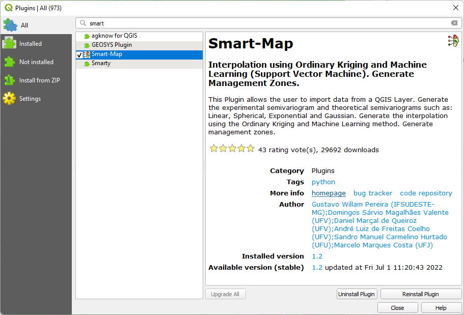
1. Install the Smart-Map plugin from the plugins manager. You probably need to install missing Python packages. Check the documentation of the plugin by clicking Homepage.
You can add those packages to QGIS using the OSGeo4W installer. Check this video:
2. After successful installation, click the  icon in the toolbar.
3. In the Smart-Map dialog stay on the Data tab and choose the NO3 layer as Input layer and choose NO3_mg_l from the drop-down list to choose the Z value. Click Import....
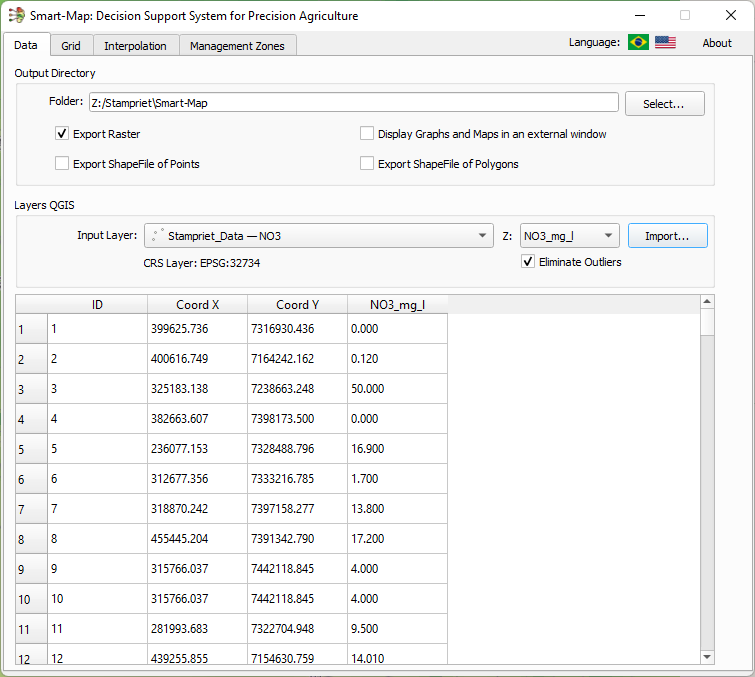
This will ingest the data and a table shows the data.
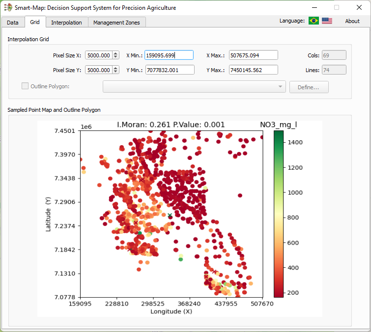
4. Go to the Grid tab. Here we can define the spatial resolution of the output raster. Set the Pixel Size X and Pixel Size Y both to 5000 m so it matches the resolution of our IDW interpolation.
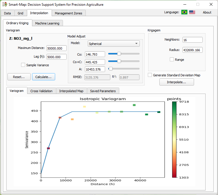
5. Go to the Interpolation tab. This is where we're going to create and fit a semivariogram. Click Calculate... to see the first result under the Variogram subtab.
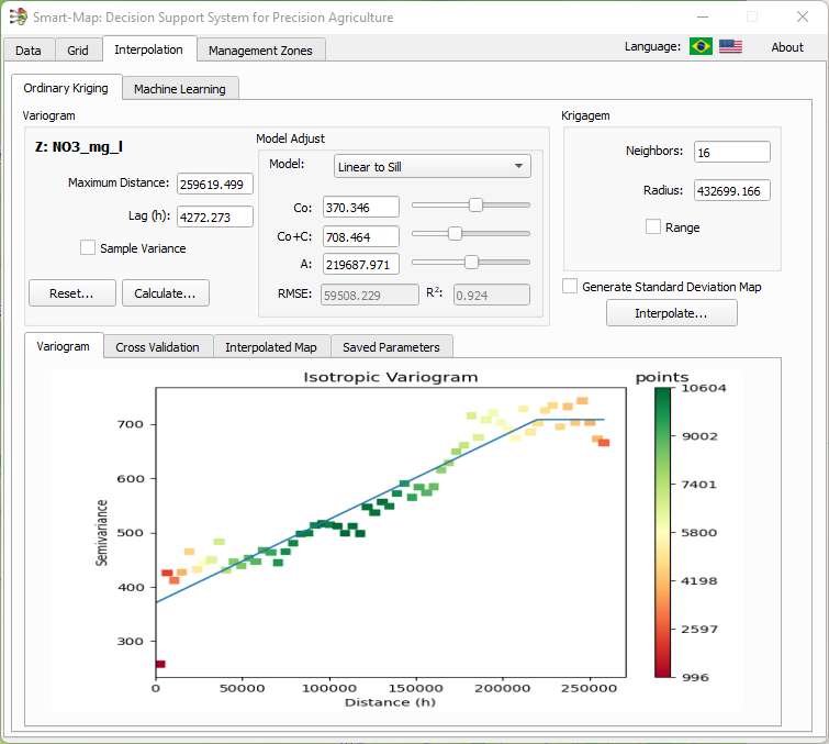
We need to change some parameters to get a better result.
This is an explanation of the settings:
- Maximum distance: maximum distance (m) for which points are considered for the variogram
- Lag(h): the distance (m) over which points are paired to calculate the semivariance
- Model: semivariogram model that is fitted using the parameters below
- Co: Nugget, which accounts for random error.
- Co+C: Sill, the maximum semivariance, which is achieved at the range distance
- A: Range, maximum distance of spatial autocorrelation
7. Play with the parameters to improve the model.
8. Once satisfied with the model, click Interpolate....
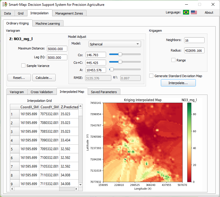
The result is shown in the dialog and the raster is loaded in the map canvas.
9. Close the dialog and click Yes in the popup to confirm.
10. Paste the style from one of the other interpolations and compare the results.
What also helps to interpret the results is to colour the NO3 points with the same gradient.
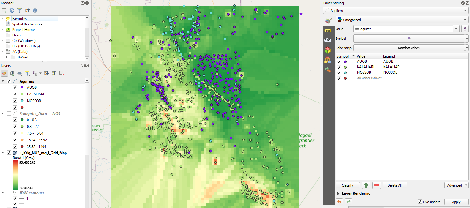
11. Move the NO3 point layer to the top of the Layers panel.
12. In the Layer Styling panel choose the Graduated renderer, use NO3_mg_l as the Value and select the same ramp as the interpolation results.
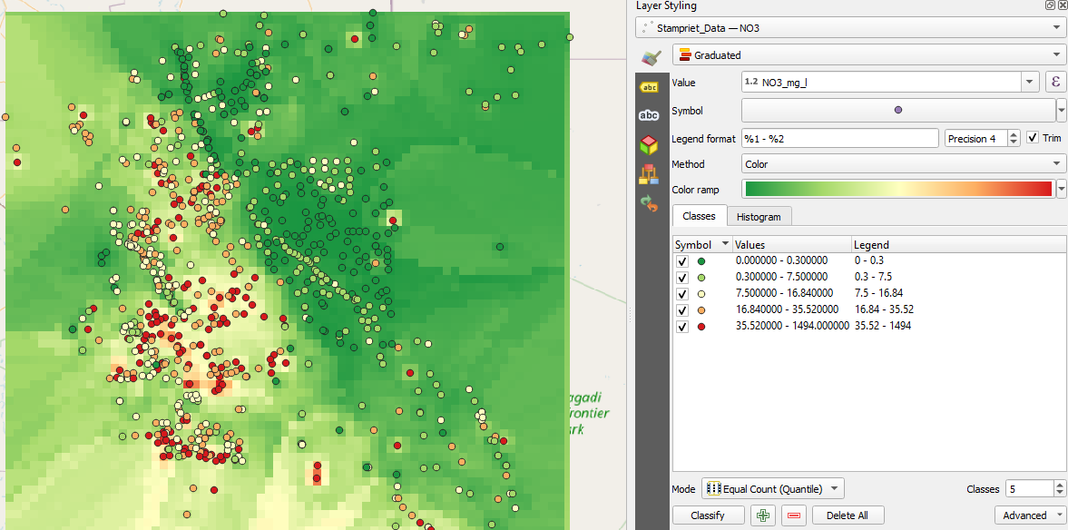
13. Adjust the class boundaries (edit the Values column) to better resemble the raster colours.
- Describe the results. Do you see patterns, what are differences?
5. Derive contour lines
We'll continue with the IDW result and will add contour lines.
An easy and quick way to visualise contour lines is to use the Contours renderer in the Layer Styling panel.
1. Make sure that the NO3_IDW layer is completely visible in the map canvas.
2. Duplicate the layer, rename it to NO3_IDW_contours and drag it above the NO3_IDW layer. Also check the box to make the layer visible.
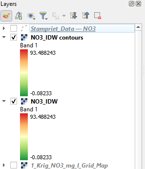
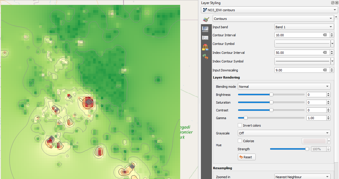
3. In the Layer Styling panel change the renderer from Singleband pseudocolor to Contours.
4. Change the Contour Interval to 10 m and the Index Contour Interval to 50 m. Change the Contour Symbol to gray.
5. With the Input Downscaling setting you can change the smoothness of the lines. Set it to 9.
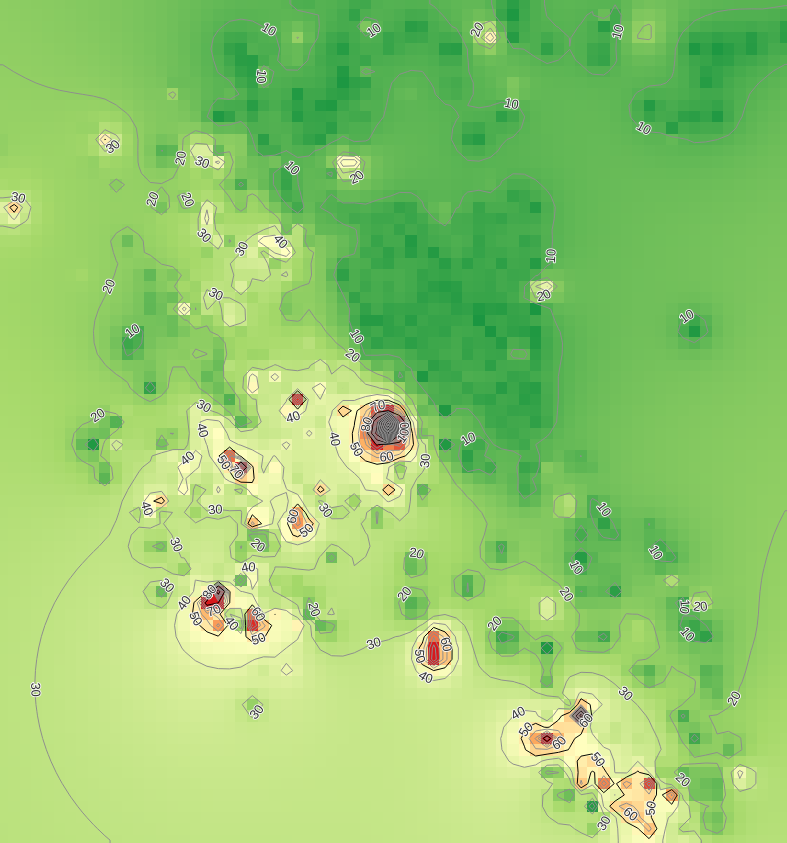
The map canvas should now look like this:
This is nice for visualisation, but not for calculations. Furthermore, we miss the labels with values of the contour lines. So, let's create a layer with contour lines.
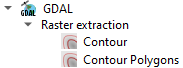
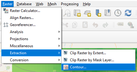
5. Choose from the main menu Raster | Extraction | Contour....
6. Choose the NO3_IDW as Input layer, change the Interval between contour lines to 10 m. Set the Attribute name to Z. Keep the rest as default and save the result as a GeoPackage with the name IDW_contours. Note that you can't save the layer into an existing GeoPackage.
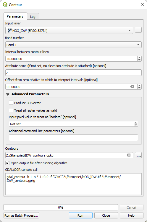
7. Click Run. Click Close after processing.
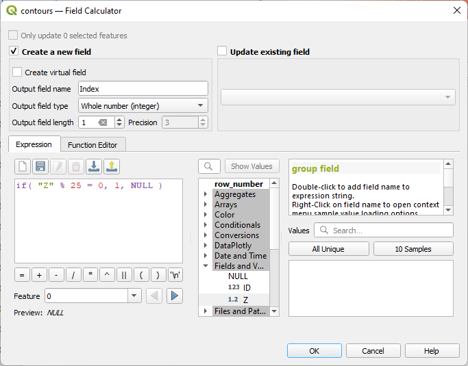
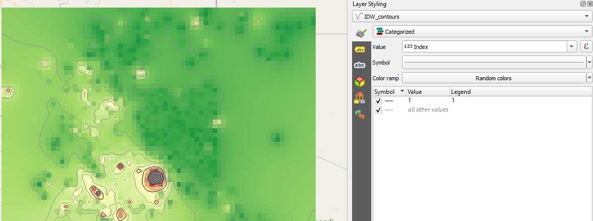
Let's style the calculated contour lines in the same way as the rendered lines.
if( "Z" % 50 = 0, 1, NULL )
 tab.
tab. tab. Change the Mode to Curved, check the On line box and uncheck the Above line box.
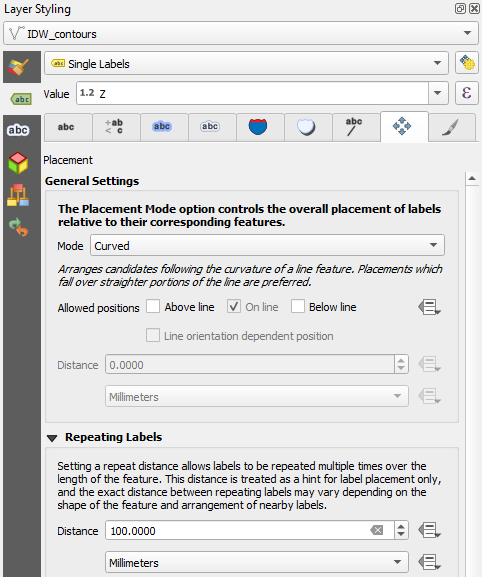
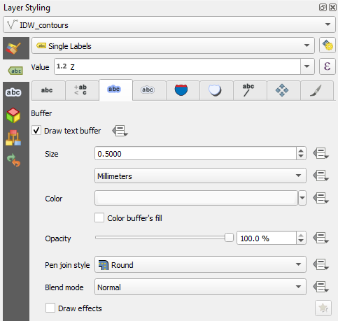
 tab. Check the box to Draw text buffer and set it to 0.5 mm. This makes the labels more readable through the contour lines.