Create an Animated Choropleth Map

Now we're ready to style the choropleth map. We need an appropriate color ramp and the borders of the countries should be visualized in a subtle manner.

Because the data contains many polygons now (each country, each year), we first need to set a filter to only show one year to set up the styling.

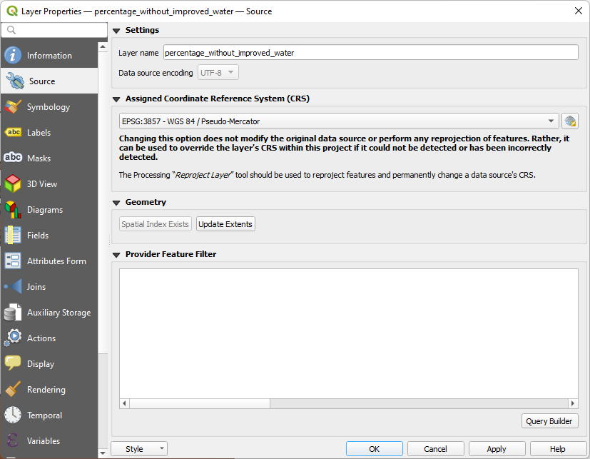
1. In the Layers panel, right-click on the percentage_without_improved_water layer and choose Properties... from the context menu.

2. In the Layer Properties dialog go to the Source tab.

3. In the Provider Feature Filter section click on the Query Builder button.

4. In the Fields box highlight the Date field and in the Values box click All to see all years.

5. Formulate an expression in the Provider Specific Filter Expression box. First double-click on the Date field to enter that in the lower box. Then click on the equals operator. Finally double-click on the year 2000.

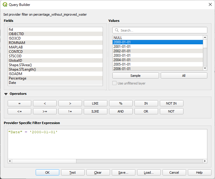
6. Click OK to close the Query Builder and click OK to close the Layer Properties dialog.

7. Make sure only the percentage_without_improved_water layer is visible, uncheck the other layers if any.

The filter icon next to the layer name indicates that you're now using a filter. When you hover your mouse over it, the expression shows.

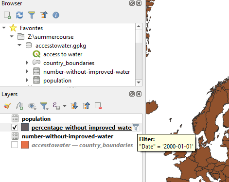
Now we'll style the filtered dataset.

8. Open the Layer Styling panel by clicking  in the Layers panel.

9. Make sure that the percentage_without_improved_water layer is the target layer in the Layer Styling panel.

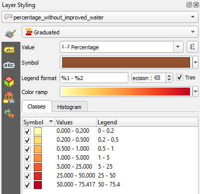
10. Use the dropdown menu to change the Single Symbol renderer to the Graduated renderer. The Graduated renderer allows you to symbolize the countries based on a numeric field.

11. For Value choose the Percentage field.

12. Click the Classify button and you will see the countries classified into the default 5 classes in your default color ramp.

13. Change the Mode to Natural Breaks (Jenks).

14. Increase the number of Classes to 7.

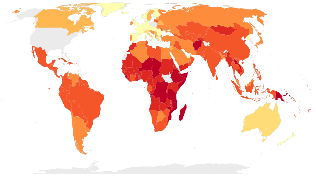
15. Use the Color ramp selector to find a nice color ramp. Here I'm using the YlOrRd ramp. The more red, the worse the condition.

16. To get nicer class boundaries, you can adjust the ranges by changing them in the Values column. In the Legend column you can edit the legend text labels.

Let's now work on the country boundaries. Some countries have nodata in some years and now their borders don't show up. We also would like to have more subtle borders.

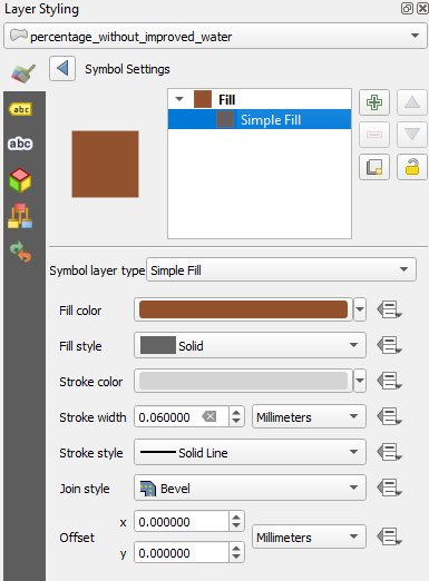
17. In the Layer Styling panel click the color bar at Symbol.

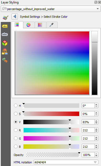
18. In the Symbol Settings click Simple Fill and and change Stroke color to a light gray (RGB 212 | 212 | 212).

19. Click  to go back and change the Stroke width to 0.06 mm.

20. Now activate the original country_boundaries layer in the Layers panel and drag it above the percentage_without_improved_water layer.

21. Make sure the country_boundaries layer is now the target layer in the Layer Styling panel.

22. Go to Simple Fill and change the Fill color to a light gray with RGB 235 | 235 | 235.

23. Go back and change the Stroke color to the same as we have used for the percentage_without_improved_water layer (RGB 212 | 212 | 212) and set the Stroke width also to 0.06 mm.

24. In the Layers panel, now move the country_boundaries layer below the percentage_without_improved_water layer and check the result.

The colors look nice now, but the projection is misleading. The project now uses the Pseudo Mercator projection, which results in disproportional areas. Let's change the projection where areas of countries are proportional.

25. Click on the EPSG code in the lower right of the QGIS window.

26. Change the projection to EPSG:8857 - WGS 85 / Equal Earth Greenwich.

Your map should now look like this:

27. Now that you have the styling set, we can clear the layer filter. Click on the filter icon in the Layers Panel to open the Query Builder. Click Clear and OK.

In the next section we'll setup the Temporal Controller.