Visualize and Animate Mesh Data
4. Extract Time Series at a Point
If we're interested in the 24 hour precipitation trend at a specific location we can extract a CSV file for that point. Let's do that for the location of IHE Delft.
We can use the Locator bar in the lower left of the window to search for addresses. It uses the Nominatim geocoder to find the location of addresses.
1. In the Locator bar type
> Westvest 7 Delft
The > indicates that you want to search for an address. You add a space and then type the address.
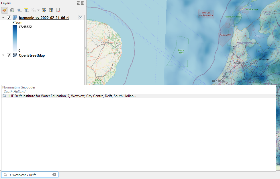
As you can see it found IHE Delft Institute for Water Education at the address.
2. Double-click on the result to zoom in to the result. Zoom out a bit to get a better view of the building.
Now we're going to digitize a point at the building, the location for which we want to report the precipitation time series. This will be a temporary scratch layer.
3. Click on  in the toolbar or select Layer | Create Layer | New Temporary Scratch Layer... from the main menu.
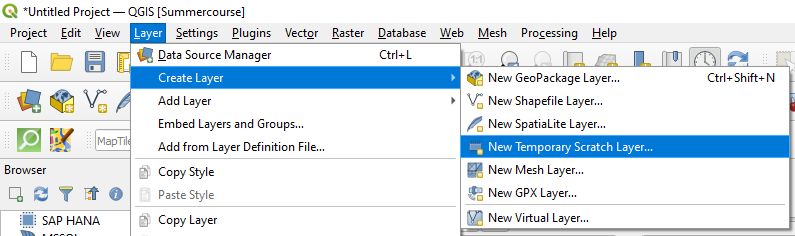
4. Change the Layer name to Location, choose Point for Geometry type and change the projection to the one from the project (EPSG:28992). We don't need to add attributes.
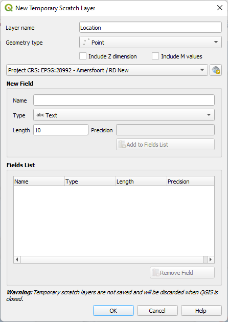
5. Click OK to add the empty layer to the Layers panel.
6. Click Add Point Feature  in the Digitizing toolbar.
7. Place the point at the IHE Delft building in the map canvas.
8. Click  to toggle off editing and save the edits.
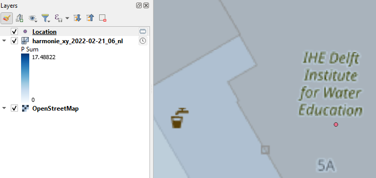
Now we can use the point to sample the precipitation values from the mesh layer.
9. In the Processing Toolbox go to Mesh | Export time series values from points of a mesh dataset.
10. Choose our mesh layer as Input mesh layer.
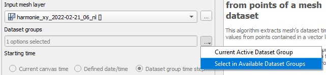
11. We're going to use precipitation and temperature. Click on  at Dataset groups and choose Select in Available Dataset Groups from the drop-down menu.
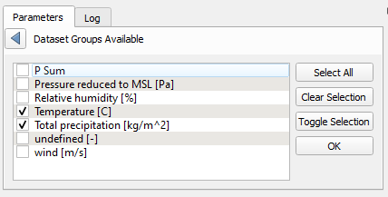
12. Check the boxes for Temperature [C] and Total precipitation [kg/m^2] and click  to go back.
13. Use the drop-down menus to select a date range from 21 February 2022, 6:00 am until 22 February 2022, 6:00 am.
14. Make sure that Location is selected as Points for data export.
15. Keep the rest as default and save the result as PandT.csv.
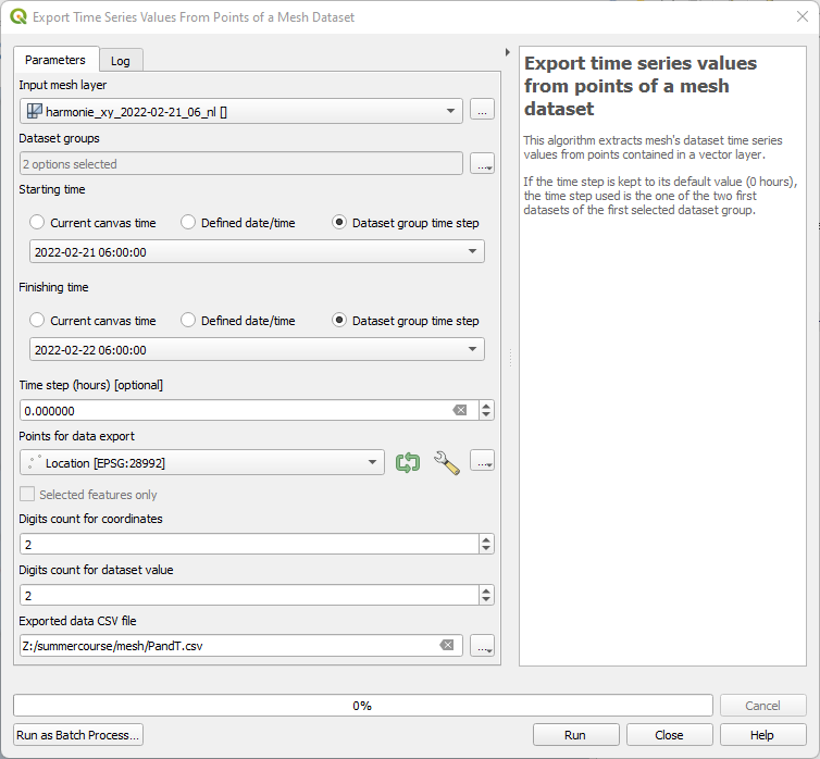
16. Click Run and Close the dialog.
17. Go to the Browser panel and drag the PandT.csv file to the map canvas (if you don't see the file, you need to click the Refresh  button).
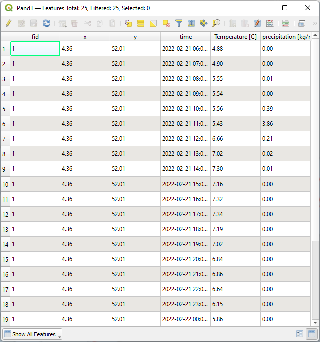
18. Right-click on the CSV file in the Layers panel and choose Open Attibute Table from the context menu.
Check the result.
In the next section we'll create plots from these time series.