Tutorial: Map Algebra with PCRaster Python
Completion requirements
5. Spatial interpolation of borehole data
To run the Jupyter Notebook of this tutorial make sure you have followed the instructions for installing Miniconda and downloading the tutorials in the previous unit. We assume that you're in the Miniconda prompt and that you're in the tutorials environment.
- Run the command from the PCRasterTutorials directory:
jupyter lab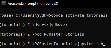
- Go to the subdirectory \PCRasterTutorials\GroundwaterInterpolation
- Click on Groundwater_level.ipynb so the Jupyter Notebook will open in a tab.
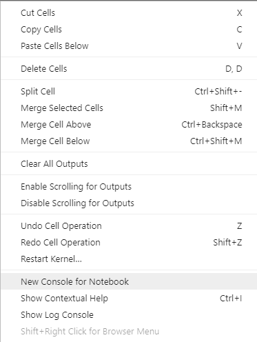
- Click right in the Jupyter Notebook and choose New Console for Notebook to add a Python Console that is linked to the notebook.
- Click the + next to the Groundwater_level.ipynb tab to add a Terminal, which you can use to navigate your file system with the CLI command that you've learned in Module 1.
- Arrange the tabs in such away (drag and drop) that your screen looks like this:
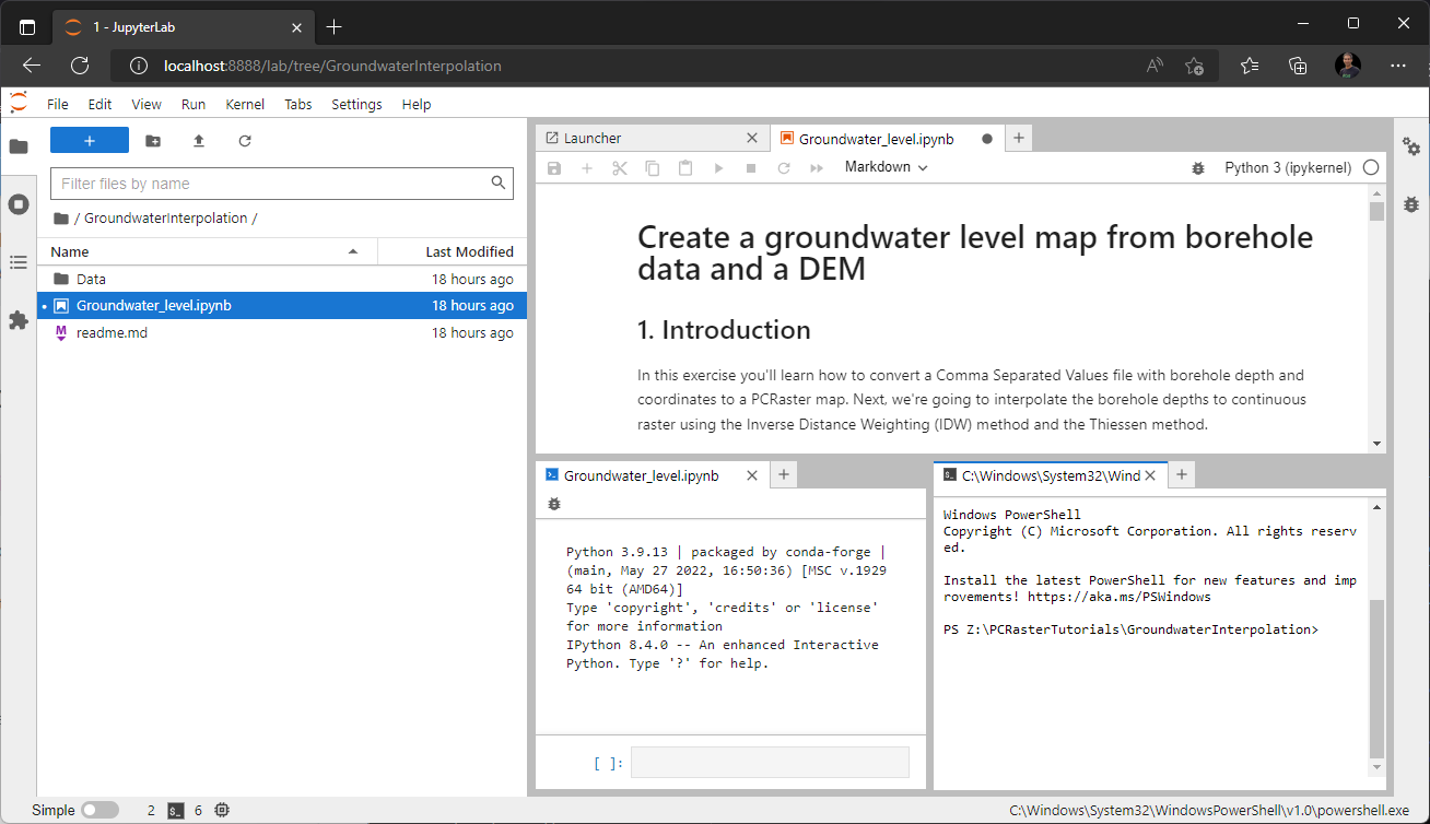
- Follow the tutorial in the Jupyter Notebook, use the Python Console to test code and use the Terminal to navigate the file system.
The tutorial is based on this QGIS tutorial and uses data from the Borehole Database in the Stampriet Transboundary Aquifer from the Orange-Senqu River Basin GIS Server. If you want to visualise the data and results in QGIS, the projection is EPSG:32734.
This video shows the whole exercise in the Jupyter Lab interface: