Fire Risk Map

A major part of remote sensing is the use of satellite imagery. Throughout the year, satellites orbit the Earth and make images of the surface. These images can be used for all kinds of applications, including the monitoring of vegetation. As we want to make a Fire Risk map, it’s vegetation we are most interested in.

During this module, we will be using imagery from Sentinel-2, which is used by the European Space Agency (ESA). For this, we will make use of the Copernicus Browser. There are multiple satellites using different types of sensors, but we want to use Sentinel-2, as it has the sensors we need for our analysis. There are a lot of different types of analyses you can perform on vegetation, but we will get into the specifics in the chapter 3. Perform Analyses.

Currently there are two Sentinel-2 satellites orbiting Earth, Sentinel-2B and Sentinel-2C. The satellites contain 13 spectral bands, named B01 to B12. B08 has two versions depending on which resolution you use. It uses a Multi-Spectral Instrument (MSI) which go from the visual spectrum all the way to infra-red, while being in a resolution of 10 to 60 meters. As our main goal is to do a Normalized Difference Moisture Index (NDMI) analysis, we are going to use a mix of B8A (B08 is only available for the 10 meter resolution) and B11. It’s going to be a bit confusing with all the different band types, and other satellites, like Landsat 8, use different names. SentinelHub is useful for referencing which bands you need to use for the analysis you want to perform, providing band names for both Sentinel and Landsat.

In the case of an NDMI analysis we use:

• B08: Near infrared (NIR).
• B11: Short wave infrared (SWIR).

If you haven't downloaded the data yet, you can download the Satellite Imagery here.

 

Importing Data

QGIS provides a few different ways to import your data. The easiest way and the only way you really need for this module is to drag it in from your file explorer.

1. Open your data folder on your device. If you used the link to download the data, it will only contain 2 files.

2. Add the B8A and B11 files into your map by selecting them in your files and dragging them to QGIS and onto your map.

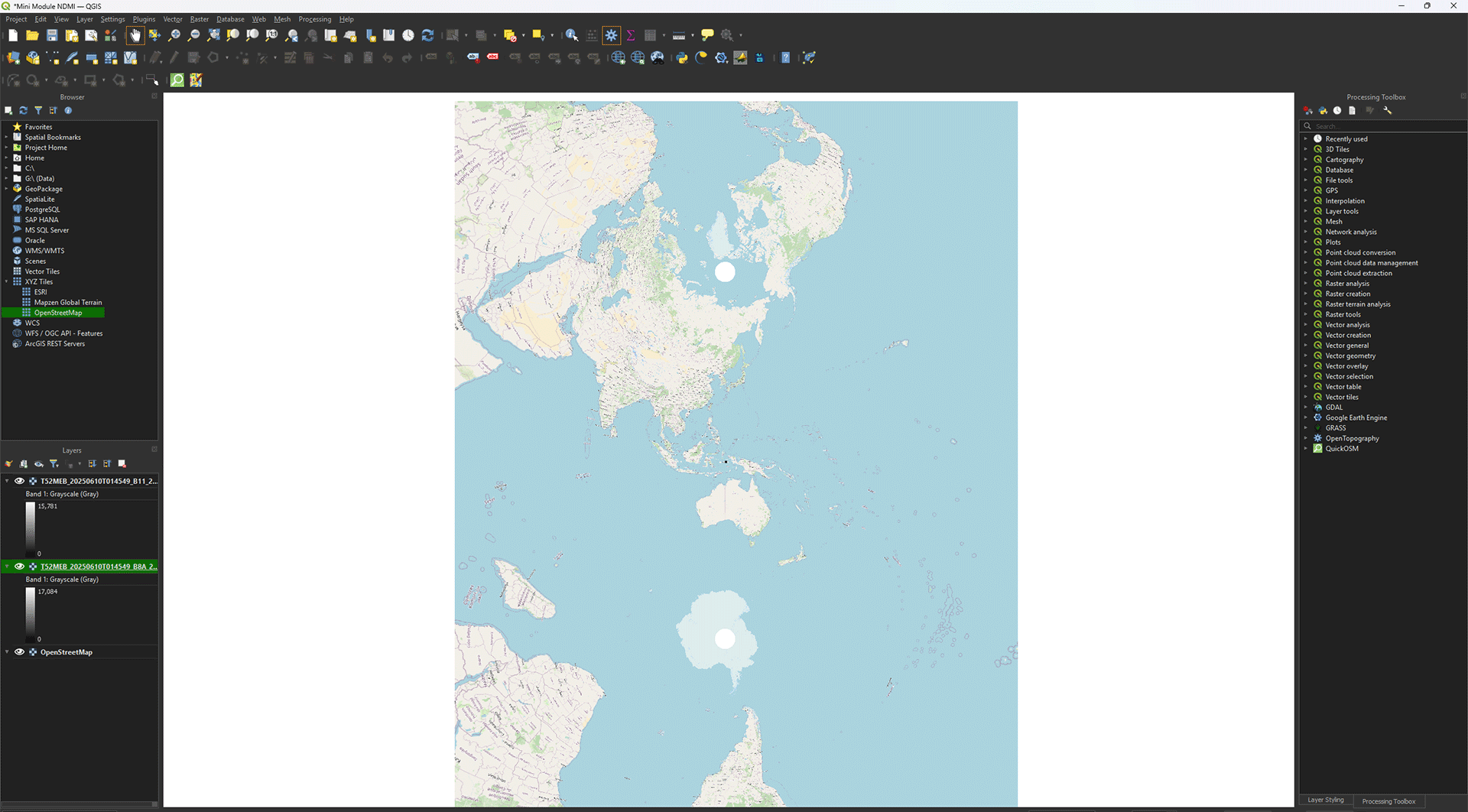
You should now see the T52MEB_20250610T014549_B8A_20m.jp2 and T52MEB_20250610T014549_B11_20m.jp2 layers in the Layers panel.

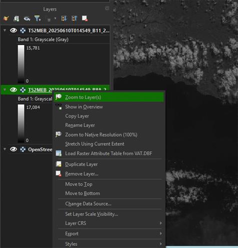
3. If the map stays zoomed out, you can right click on the layer and press Zoom to Layer(s).

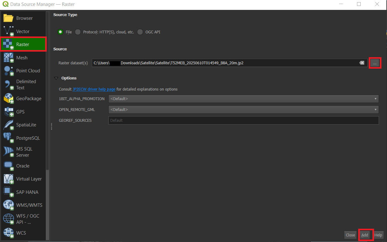
Another way to import data is via the Data Source Manager in QGIS. This can be helpful if you have very specific data types that need the certain settings to import correctly, like CSV (usually used in Excel) data. You can choose for yourself which way you prefer, for this module we won't need to import settings so it does not matter how you import the data.

After clicking on Data Source Manager you will get a pop up screen, here you can select what kind of data you want to import on the left. In the case of the satellite bands, we want to import Raster data. You can click the three dots on the right of the Raster dataset(s) to import the data you want from your computer. After selecting the file you want it will show up in the Raster dataset(s) box. Click Add to load the data from the file into your map.

Or you can find your data via the Browser panel as well. In the browser panel you will see your own files, you can search within these files for the place where you saved the data you want and drag it onto the map.

 

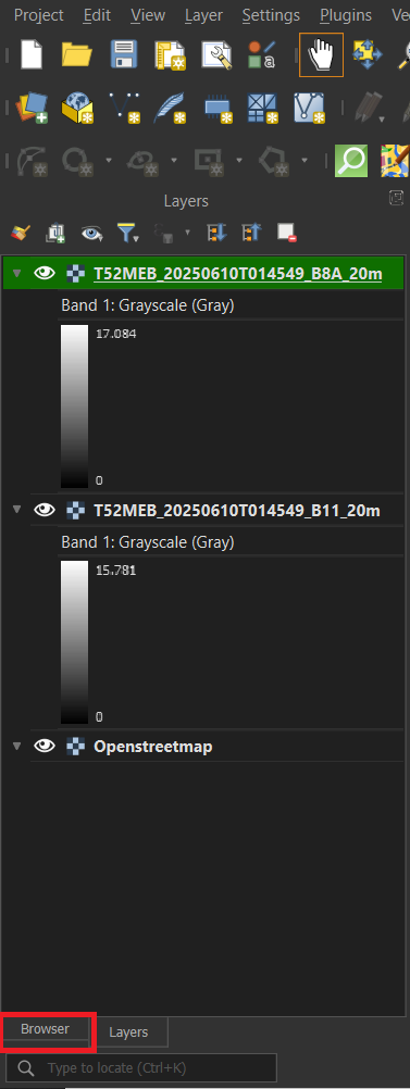
Another important thing about working with QGIS, is that it will often save newly created layers as Temporary Layers. The ones we just imported are Permanent layers, as they are saved on your device, while Temporary Layers are only, as the name suggests, temporary. You can recognize them by this symbol.

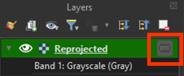
This means that the file will be deleted when you close QGIS, even if you saved the Project. You can right-click on the Temporary Layer > Export > Save as. Save it on an easy to find location. Once done, you can delete the Temporary Layer from the Layers panel.

 

Reprojecting

When importing data into QGIS, it will often times place the data on the wrong CRS. In chapter 2.1, we set the CRS of the project to EPSG: 32752. All data that gets imported into QGIS for this project needs to be placed in the same CRS, otherwise your map can be slightly blurry and distorted. Like your map is now if you look very closely. This is because the layers we just imported are projected on the WGS84 CRS instead of the projects CRS. To fix that we are going to reproject the layers first, because otherwise the resampling we need to do later will fail and break our data.

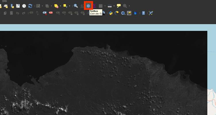
1. If you don’t have the Processing Toolbox open already, go to the cogwheel symbol on the top of the screen.

 

2. Go to the Processing Toolbox and search for Warp (reproject) under GDAL > Raster projections. Double click to open the tool.

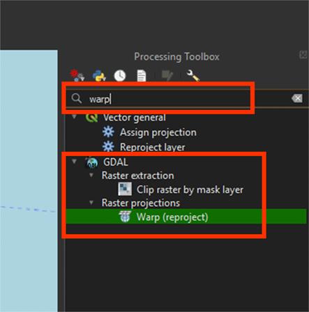
Note: The standard Reproject tool is meant for vector layers. We are reprojecting a raster layer, so we need to use Warp instead.

A new window will open. Here we can change the settings and reproject our layers.

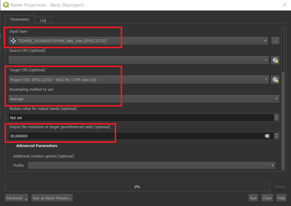
3. On Input layer, select the T52MEB_20250610T014549_B8A_20m.jp2 layer.

4. Set the Target CRS on EPSG: 32752.

5. Set Resampling method to use on Average This will take the average values and create new pixels based on them.

As we are using multiple data sources, we need to make sure that all the rasters are the same resolution. A good rule to follow is that you always resample all the data to the data with the lowest resolution. It’s easy to remove data, but difficult to create data from a low-resolution source. We will use a Digital Elevation Model, which only goes to a resolution of 30 meters. Our satellite imagery is 20 meters. This means we are going to resample it to 30 meters.

6. Under Output file resolution in target georeferenced units, set the value on 30. This will convert our 20 meter resolution to 30 meters.

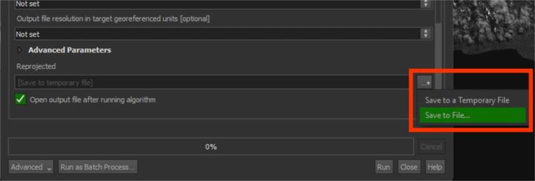
7. Scroll down to the bottom of the pop-up to find the saving button. Under Reprojected, press the arrow button and save the file in an easy to find location. Name the file B8A_Reprojected, then click Run.

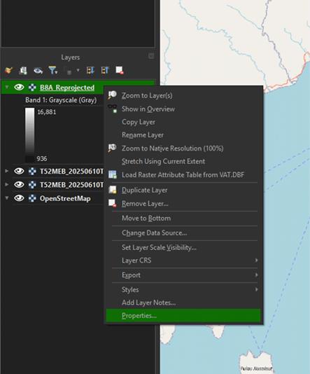
The layer is now correctly reprojected. You can check if the CRS is correct by right clicking the B8A_Reprojected layer > Properties > Source. It should say EPSG: 32752. Under information, you can see the resolution. It should say 30. 

Note: If you can't see the layer, try rearranging your layers in the Layers Panel. You can do this by dragging the layers above or below each other or you can deselect the Eye next to the layer’s name to make it invisible.

 

8. Follow the same steps to reproject the T52MEB_20250610T014549_B11_20m.jp2 layer, starting from step 2, by using the Warp tool. Save the file the same way and name it B11_Reprojected.

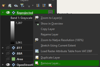
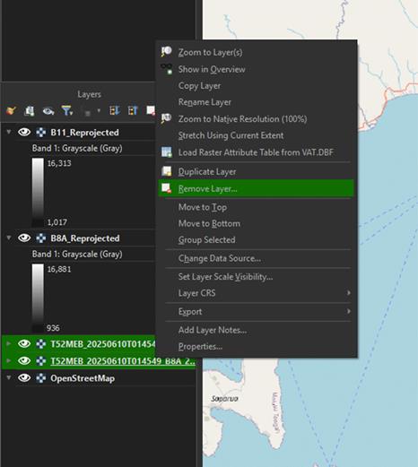
You can delete the imported layers, as we don’t need them anymore. Right click on the layers and press Remove Layer.

 

Clip Study Area

As we want to analyze a small area, we want to make our data a lot smaller as well. If we use the entire image to do our analyses, we will dedicate a lot of time and compute power to something that we don’t need. For most projects, we make use of an area of interest. This is usually done with a polygon layer. You can get them from a variety of sources, like a country’s borders, but for this module we will create our own.

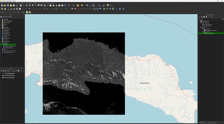
This area is what we are going to use. Make sure the B8A_Reprojected layer is visible.

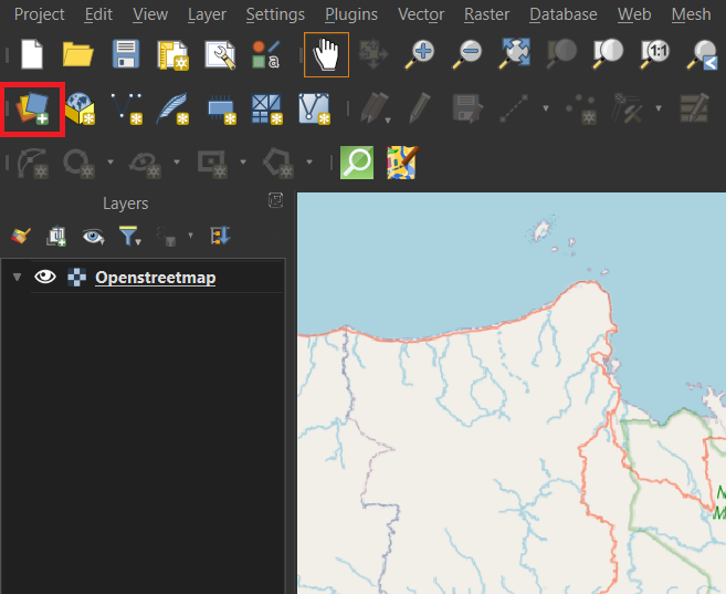
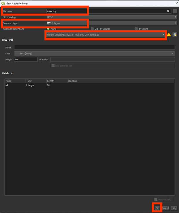
1. Click the New Shapefile Layer to create a new polygon.

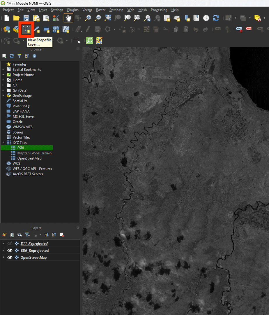
Any polygon, line, or point will need to be saved into a Shapefile. Shapefiles are made of vectors, meaning they are infinitely sharp, as they don’t use pixels like a raster does. A lot of data uses Shapefiles, so you’ll come across them quite often. We will delve deeper into vector layers later.

2. Name the file Area and press the ‘…’ button to save the layer on an easy to find location.

3. Select Polygon under Geometry type.

4. Make sure that the CRS is set to EPSG: 32752.

5. Click on OK.

 

Now, we will see a new layer in our Layer panel, but nothing on our map. We will need to create our polygon.

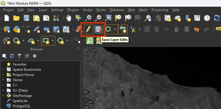
6. Click on Toggle editing and make sure the Add polygon and Rectangle from the extend buttons are selected.

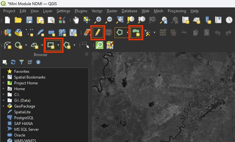
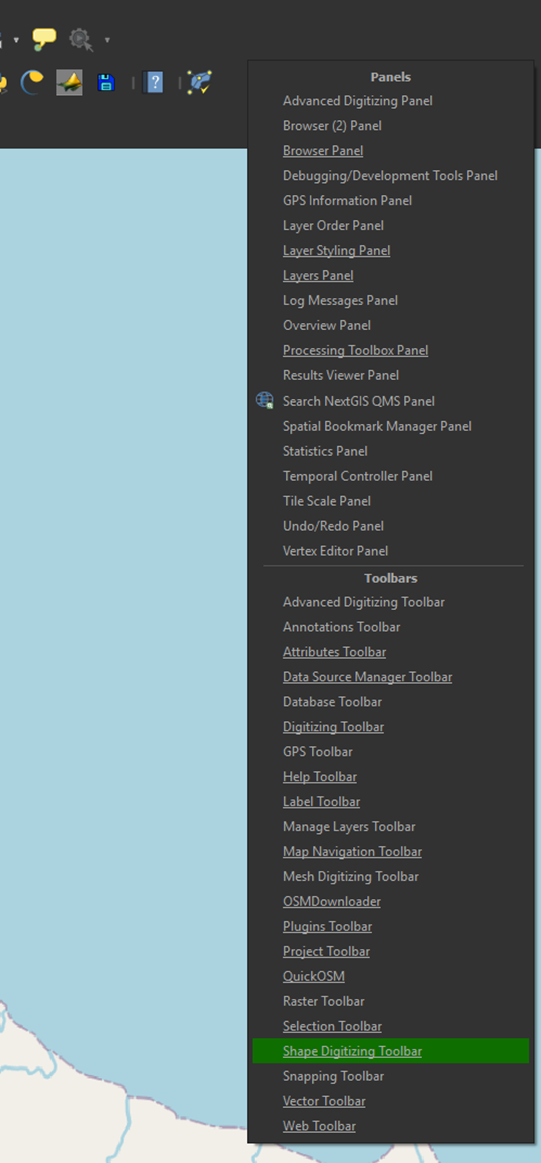
Note: If the options don’t show up, you can add them by right clicking on the toolbar and selecting Shape Digitizing Toolbar.

7. Click and create a rectangle around the area of interest. Right click to draw the polygon. The shape doesn’t have to be the exact same as the example.

You’ll get a pop-up to give the polygon a value. You can keep it on NULL, as the data in the polygon is not important for our needs, but you can also fill it in with a number, like 1. 

Once the polygon is created, you’ll see it appear on the map. If you want to redo the polygon, you can press ctrl + z and draw the polygon again.

8. Press the Save icon. Make sure you always do this when working on polygons. You can easily lose the data if you forget. Once you’re happy with the polygon, press the Toggle editing button to stop editing the Shapefile.

Now that we have a study area, we can start clipping the rasters and make them all the same size. 

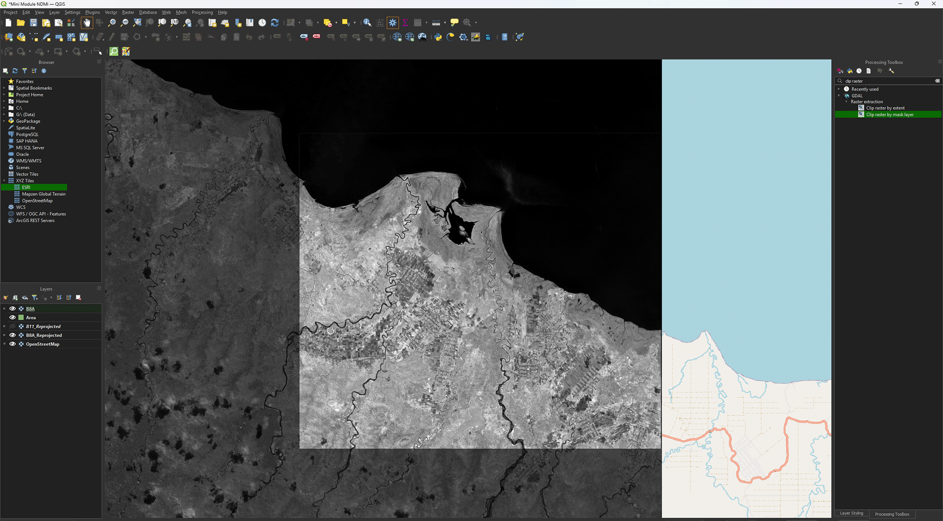
9. Go back to the Processing Toolbox. Search for Clip raster by mask layer under GDAL > Raster extraction. Double click to open.

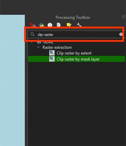
Note: The standard Clip tool is only meant for clipping shapefiles. We need the Raster extraction tools to clip rasters specifically.

11. In the window, set the Input layer to the B8A_Reprojected image.

12. Set Mask layer to Area. This will clip the raster into the polygon we just made.

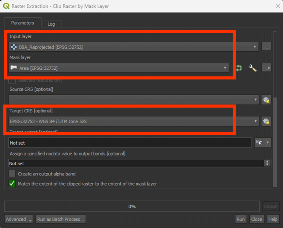
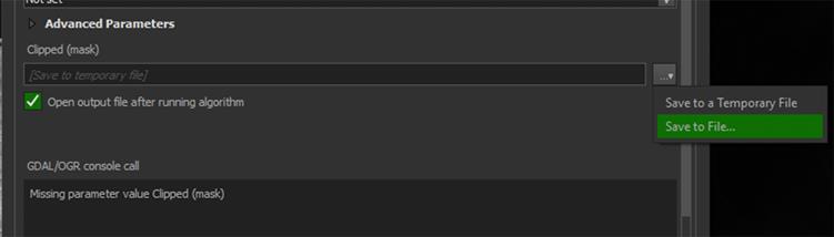
13. Sroll down and go to Clipped (mask) and press the arrow button > Save to file > name it B8A. Save it to an easy to find location. Then, Run the tool.

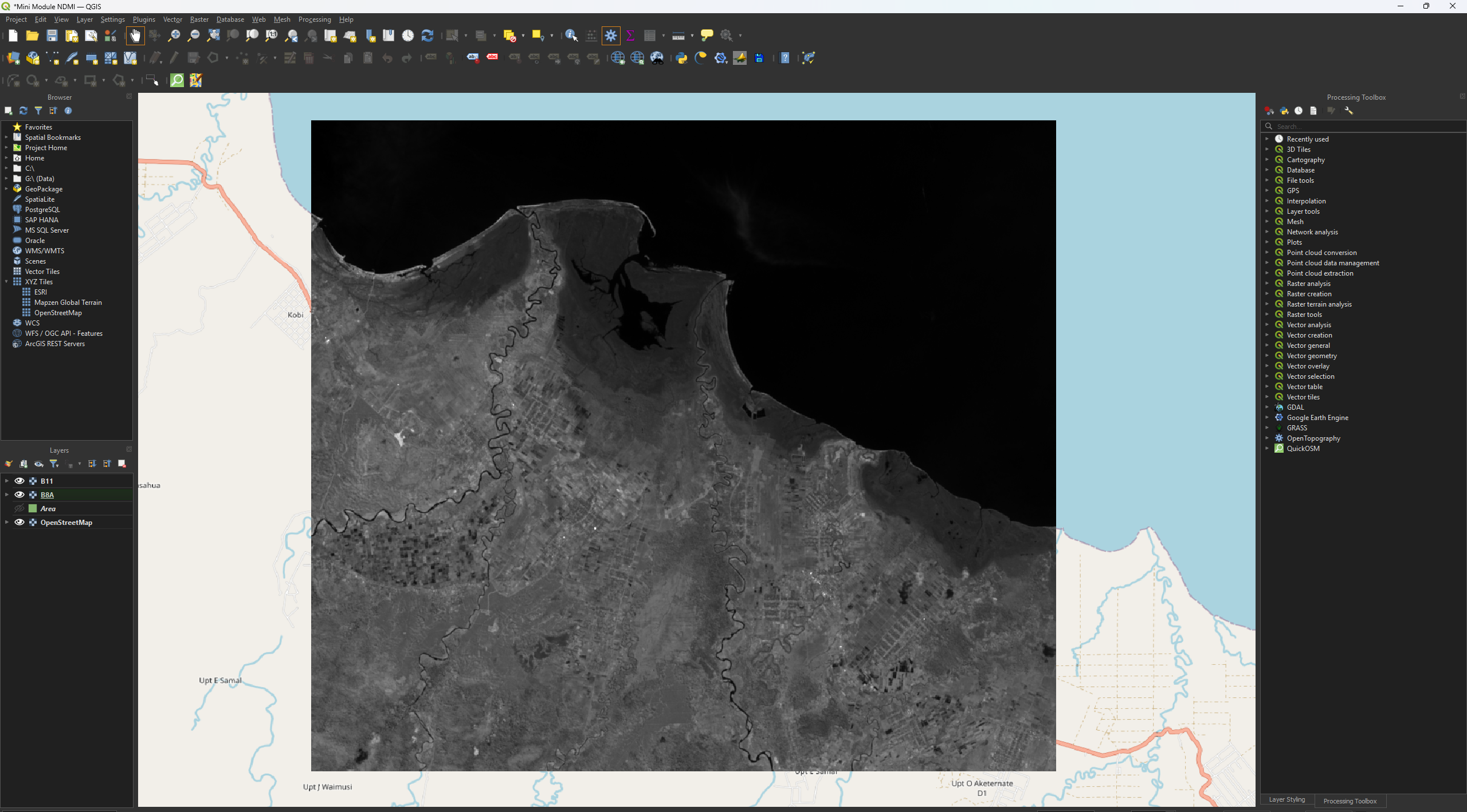
The image should now only show the study area.

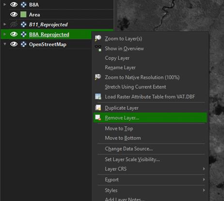
We don’t need the B8A_Reprojected image anymore, so we can delete it from our project.

14. Right click the layer we used to clip > Remove layer.

Note: As we saved the layer earlier, you can always add it back into QGIS by dragging it from your folder.

Repeat these steps, starting on step 9, to clip the B11_reprojected image you created as well. Once clipped, save the layer as B11 and delete the B11_reprojected layer.

You have now reprojected and clipped the B8A and B11 layers. Before we continue, save your project by pressing the save icon or pressing ctrl + s.