Fire Risk Map

Below there is some information about everything you need to know before you start the Extra Assignment. Make sure you read everything. Most of the steps are the same, but there are some things to keep in mind to get to the correct result. Good luck!

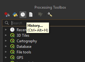
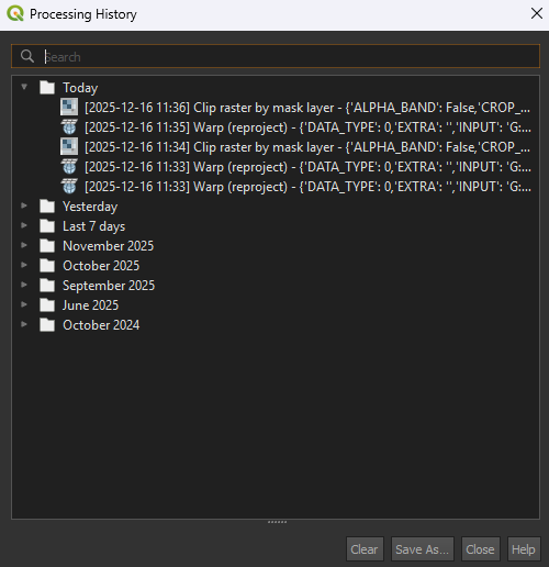
Tip: At the top of the Processing Toolbox, there is a History icon. This lets you see all the analyses you have performed. You can double click on an analysis/tool and it will have saved all the settings. This is helpful if you have to redo some steps. Make sure that you set the correct layer as the input and save the layer with the correct name, as to not accidentally overwrite a different layer.

 

 

Project and Coordinate System

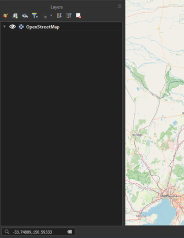
After starting a new project, you can use these coordinates to find the location: -33.74889,150.59333. Paste these coordinates in the search bar below the Layers panel.

 

Before you start on the analysis, you have to choose the correct coordinate system. We can’t use the same one we used for the main module. As we are in Australia, New South Wales specifically, we can use GDA2020 / NSW Lambert EPSG: 8058. Make sure you import the OpenStreetMap basemap under XYZ Tiles first, otherwise the CRS may revert back, and you have to apply it again. Every time you have to set the CRS anywhere, you’ll use EPSG: 8058. The resolution will still be the same at 30m.

 

Satellite imagery

Like the main module, you can get the satellite imagery from the download folder. However, if you want, you can try to download the data yourself. In 6.1. Satellite Imagery, the process of downloading satellite imagery is explained. Do make sure you download the images from the correct location, which is Sydney, New South Wales, Australia. We will still use Sentinel-2 and the B8A and B11 layers. We want to look at the fire season of Australia, which for the Sydney area falls somewhere between October to February. Try to find something around December or January to be sure. Set the Time Range from 2024-10-01 to 2025-02-28.

Depending on the data you’ve downloaded, you may have to combine images using the Merge tool. This works the same way as you have done with the Land Cover layer in the main module

 

DEM

Make sure you use the correct CRS for all the layers. For the Elevation download, you don’t have to get a new API key, you can always use the same one. The download may be a bit wonky and not fitting your study area. If that happens, you can use the Clip raster by mask layer tool to clip it nicely into your study area.

 

Land Cover

You may have to use the Merge tool if you have data that doesn’t fully cover your study area. It’s the same process as you did for the Land Cover layer in the main module. You can also download the data yourself by going to 6.2. Land Cover.

 

Roads and Buildings

Depending on the size of your study area, there could some data missing of the OSM data, mainly the buildings. If you have a large study area, the download can take a while.

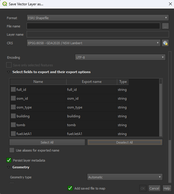
When working with larger OSM layers, you might run into some issues when you are saving the layer. To circumvent this, skip saving the layer when using the Reproject and Dissolve tool and use a Temporary layer instead. When you created the Temporary Dissolve layer, right click on the layer > Export > Save Feature As… and save it as a Shapefile (SHP). Then under Select fields to export and their export options, press the Deselect All button. This will remove all the features from the layer (we don’t need them for the analysis).

This should save the layer correctly. If you are still running into issues, you can download the layers here[TH3] .

 

NDMI

Calculating the NDMI is the same process as the main module.

 

Slope

Unless you have a part of the ocean in your study area, you don’t have use the Fill no data tool for this analysis.

 

Distance to Built-Up Area

As we have discussed in the main module, creating using the Multi-ring buffer can be very heavy. If you have a large study area, consider using the other method with the Proximity tool for creating a buffer. For the buildings, it’s recommended to use the Proximity tool as well.

 

Weighted overlay analysis

As we are using this Extra Assignment as practice, we aren’t going to delve into choosing the correct values for our Weighted Overlay Analysis. You can use the same scores as we used in the main module. There are some things to keep in mind, however:

 

Slope

The results of the Slope analysis are probably a bit steeper than in the main module. If your slope degrees go above 30, you’ll need to set a limit. Above 60 degrees, the slopes become too steep, so we can value these areas as a score of 0.

The bottom 2 rows in your table should look like this:

Minimum	Maximum	Value
30	60	10
60	9999	0

 

Land Cover

There is a good chance that some land cover types aren’t found in your study area, like mangroves. The data will still contain naming for mangroves, but no pixel is coloured that way. This is the same as how we didn’t have any snow and ice in our main module study area. You can keep the scores the same as the main module, as mangroves shouldn’t appear anyway, it won’t affect the results.

 

Calculate map

You can use the same formula as the main module.

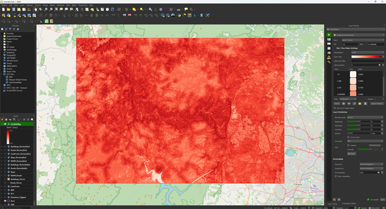
The final result should look something like this:

 

Risk map visualisation

The final result of the grid should look something like this:

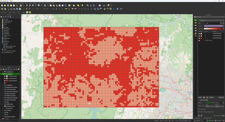
This is a pretty large area, so you can adjust the Reclassify. Just for trying something different, you can give the Fire Risk Map a classification of 1 – 10 instead of 1 – 4.

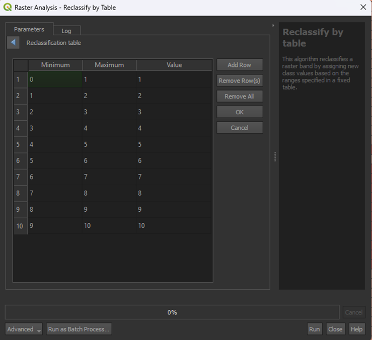
That results into this:

 

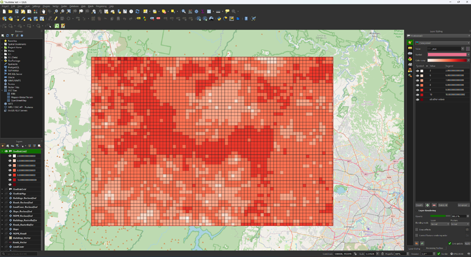
This isn’t a very good classification, but it shows that you can change what the classification is depending on what you want to show. For this data, a risk level from 1 to 4 may not be detailed enough, while it worked for the main module.