Tutorial: Remote Sensing Image Classification with QGIS

Random Forest is one of the most versatile and widely used machine‑learning algorithms for remote sensing. Instead of relying on a single decision tree, a Random Forest builds many trees, each trained on a slightly different subset of the data, and then lets them “vote” on the final class. This ensemble approach makes the method remarkably robust: it handles noisy training data, reduces overfitting, and performs well even when classes overlap in spectral space.

For remote sensing applications, Random Forest is especially attractive because:

• It works well with high‑dimensional data, such as multispectral or hyperspectral imagery.
• It can model complex, non‑linear relationships between spectral bands and land‑cover classes.
• It provides measures of variable importance, helping you understand which bands or indices contribute most to the classification.
• It requires minimal parameter tuning, making it accessible for beginners while still powerful for advanced users.

More info can be found here.

Let's configure the Random Forest classifier in SCP.

1. In the main menu, go to SCP | Band processing | Classification.
   
2. Under the Algorithm section click on Random Forest to expand the configuration settings.

You’ll see several parameters you can adjust. Each one influences how the forest of decision trees is built and how your final land‑cover map is produced.

Number of Trees

• Defines how many decision trees the algorithm will grow.
• More trees generally improve stability and accuracy because the “forest” can average out noisy or biased trees.
• Typical values range from 100 to 500, but SCP allows you to go higher if needed.

Minimum number to split

• Sets the minimum number of samples required to create a new split or leaf.
• Higher values make trees more conservative and reduce overfitting.
• Lower values allow more detailed splits but may capture noise.

Max features (per split)

• Determines how many predictor variables (bands, indices, etc.) each tree considers when splitting nodes.
• Randomizing this selection is what gives Random Forest its strength.

When you run a Random Forest classification in SCP, you’ll see a few extra options that help the algorithm deal with tricky situations. One‑Vs‑Rest tells the classifier to look at each class separately: it learns to distinguish one class from all the others, which can help when some classes are harder to separate.

Cross validation is a built‑in way for SCP to check how well your model is likely to perform on new data. It repeatedly trains and tests the classifier on different subsets of your samples, giving you a more reliable accuracy estimate without needing a separate validation set.

If your training data is unbalanced, for example, if you have many samples for vegetation but only a few for water, you can turn on Balanced class weight. This gives smaller classes more influence during training so they aren’t overshadowed by the larger ones.

SCP can also find the best estimator for you. This means it automatically tries different combinations of Random Forest settings and picks the one that performs best. It’s a helpful shortcut when you’re not sure which parameters to choose.

Finally, you can create a classification confidence raster, which shows how confident the model is about each pixel. High values mean the trees in the forest strongly agreed on the class; lower values highlight areas where the model was uncertain. It’s a great way to visualize where your map is most reliable and where you might want to be cautious.

Let's configure some settings for our first try.

3. Keep the number of trees as default so the preview in the next section will calculate fast. After that we'll increase the value. 300-500 is typically used.

4. Toggle on One-Vs-Rest. This helps separate similar crops by giving each class its own focused model. It reduces confusion when spectral signatures overlap.

5. Toggle on Cross validation. This will give us an internal accuracy estimate.

6. Toggle on Balanced class weight. In our case some classes have many more training samples than others. It ensures that minority classes aren't ignored.

7. Toggle on Calculate classification confidence raster. In this way we can identify ambiguous pixels.

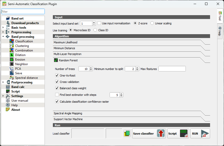
8. Close the dialog.

Now we've configured the classifier, we can apply it to our image in the next section.